6.3 State-space models with imposed displacement and acceleration
In order to be able to impose a displacement or acceleration instead of a mechanical load, the displacement vector {q} is divided in two contributions:
where {qI} is the part of {q} on which either a displacement or an acceleration need to be imposed (I is used as a reference to "interface"), and {qC} represents the remaining dofs where no displacement or acceleration is imposed. As will be discussed later, different choices can be used for [TI] and [TC].
We assume a general form of these matrices where for the degrees of freedom related to imposed displacement or acceleration in {q}, the associated lines in [TC] must be all zeros, and for the [TI] matrix, all zeros except one on the column related to this degree of freedom. In doing so, the degrees of freedom related to {qI} are the physical displacements of the structure where the displacement or acceleration needs to be imposed.
If the full finite element model of the structure is used, matrix [T]C is a N × N identity matrix from which the columns corresponding to the imposed dofs have been removed.
The strategy to choose matrix [TI] will differ for the case of imposed displacement and acceleration, as will be detailed below. Using (20), the equations of motion (2) become (u(t)=0)
and after premultiplying by [TC]T and putting the unknown displacements {qC} to the left-hand side of the equation, we get
where [MCC], [CCC] and [KCC] are the mass, damping and stiffness matrices with fixed boundary conditions at the degrees of freedom corresponding to {qI}. The subscript C stands for constrained, as the equations of motion in (22) correspond to a dynamic problem for which the degrees of freedom corresponding to the imposed motion are fixed, and the imposed displacement, velocity or accelerations correspond to an equivalent mechanical force vector.
As such, it is difficult to build a state-space model from these equations, whether for imposed displacement or acceleration, because only one of the two is imposed and the other is unknown.
6.3.1 State-space models with imposed displacement
For imposed displacement, the typical choice for [TI] consists in taking a matrix which is limited to the degrees of freedom where the displacement is imposed. All terms on the rows corresponding to the non-imposed degrees of freedom are therefore equal to 0. In this case, the forces acting on the structure are limited to the degrees of freedom which are coupled to the interface through the stiffness, mass, and damping matrices. If the mass matrix is diagonal, there is no such coupling, and if it is not, the coupling is very weak, so that the forces related to inertia can be neglected. This is also the case of the damping forces, as long as the damping is small. In such a case, the equations become
where now the forcing vector is only a function of the imposed displacements. With this formulation, a state-space model can be built using the approach detailed in section 6.1.2, where normal modes of the system with the imposed dofs set to 0 and a static correction to − [TC]T [K] [TI] is added. The displacement at the imposed dofs can be directly recovered using the [d] matrix if a sensor is defined at these location, using matrix [T]I.
Note that in (23), there are as many inputs as there are degrees of freedom in {qI}. This can be simplified to a single input using an expansion vector such that:
where q0 is now a single input scalar displacement to the system, and the right-hand-side of equation (23) reduces to a single vector multiplied by the input displacement q0. The number of necessary static responses to build the state-space model is therefore also reduced to one instead of the number of degrees of freedom in {qI}.
The construction of a state-space model with imposed displacement is illustrated below on the same example of the concrete tower. The function fe2ss is used to build directly the I/O state-space model from the finite element after defining properly the input (horizontal imposed displacement Uimp) and the output (displacement at the top of the tower d−top).
In  d_piezo('TutoPzTowerSSUimp-s1')
, the mesh is built and a horizontal displacement is imposed at the basis of the tower.
d_piezo('TutoPzTowerSSUimp-s1')
, the mesh is built and a horizontal displacement is imposed at the basis of the tower.
Then in d_piezo('TutoPzTowerSSUimp-s2')
, the transfer function between Uimp and d−top is computed using low-level calls using only the stiffness term in the excitation term, or both the stiffness and mass terms.
[model,Case] = fe_case('assemble NoT -matdes 2 1 Case -SE',model) ;
K0 = feutilb('tkt',Case.T,model.K);
F1 = -Case.T'*model.K{2}*Case.TIn;
F2 = -Case.T'*model.K{1}*Case.TIn;
w=linspace(0,100,512);
for i=1:length(w)
U0(:,i)=Case.T*((K0{2}*(1+0.02*1i)-w(i)^2*K0{1})\(F1-w(i)^2*F2));
U1(:,i)=Case.T*((K0{2}*(1+0.02*1i)-w(i)^2*K0{1})\F1);
end
CTA = fe_c(model.DOF,21.01); u0 = CTA*U0; u1 = CTA*U1;
C1=d_piezo('BuildC1',w'/(2*pi),u0.','d-top','Uimp'); C1.name='M and K';
C2=d_piezo('BuildC1',w'/(2*pi),u1.','d-top','Uimp'); C2.name='K only';
ci=iiplot;iicom(ci,'curveinit',{'curve',C1.name,C1;'curve',C2.name,C2});
iicom('submagpha')
d_piezo('setstyle',ci);
Figure 6.5 shows that the two curves match perfectly, meaning that the inertial term can indeed be neglected for the excitation, allowing to build an accurate modal state-space model with a static correction with the stiffness term only.
This is the approach used in SDT and illustrated in d_piezo('TutoPzTowerSSUimp-s3')
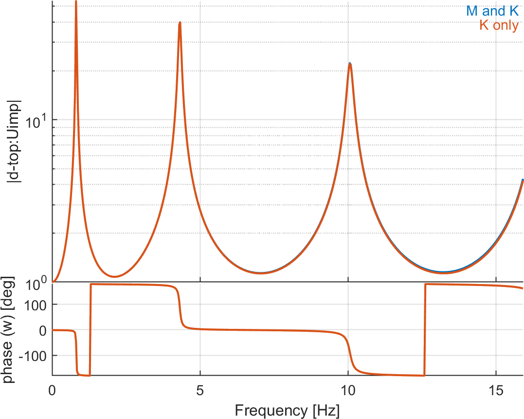
| Figure 6.5: Transfer function between horizontal displacement at the bottom/top of the beam using the full model, the loading takes into account both the mass and stiffness terms, or only the stiffness term (dtop/Uimp) |
sys=fe2ss('free 5 5 0 -dterm',model);
C3=qbode(sys,w,'struct-lab');C3.name='fe2ss-5md+st'; C3.X{2}={'d-top'};
ci=iiplot;iicom(ci,'curveinit',{'curve',C1.name,C1;'curve',C3.name,C3});
iicom('submagpha')
d_piezo('setstyle',ci);
Figure 6.6 compares the frequency response functions used with the full model and direct computation, and using a state-space model with 5 modes and a static correction for the stiffness loading term. The match between the two is excellent.
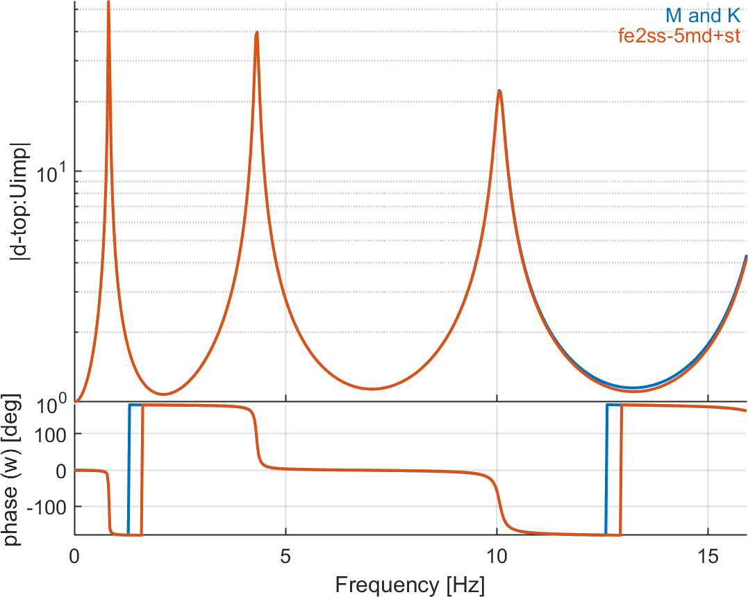
| Figure 6.6: Transfer function between horizontal displacement at the bottom/top of the beam using the full model and the reduced state-space model with 5 modes, the loading takes into account only the stiffness term (dtop/Uimp) |
6.3.2 State-space models with imposed acceleration
In the case of imposed acceleration, it is common to write the problem in terms of relative displacements with respect to the base motion, in which case matrix [TI] is not anymore limited to the imposed displacements. The approach consists in choosing [TI] as the static response to imposed displacements, so that it relates to all dofs in the structure. Let us assume that the dofs of the structure are rearranged so that the matrices can be decomposed in four blocks as previously :
where the index I corresponds to the imposed dofs. [TI] is then given by the static expansion of the imposed displacements:
where {q0} represents the spatial shape of the imposed acceleration at the specific locations.
Such a representation is general enough to take into account base excitation problems where the excitation of the base is uniform and in a single direction, such as a uniform translation of the base. In this case, [TI] represents the rigid body translation of the structure in the direction of the base motion, and {qC} is the relative motion of the structure with respect to the translation of the base. The general approach allows also to impose a combination of the six rigid-body modes of the structure. In this case, the quantity that is withdrawn from the global motion in order to represent the relative motion is different at each location in the structure in the case where rotational rigid body motions are present in the base excitation.
Lastly, the approach also allows to take into account base excitations which induce a deformation of the basis, in which case [TI] is not a rigid body motion but the static expansion of the imposed displacements on all other dofs of the structure (which reduces to rigid body motions if the imposed displacement is a translation and/or rotation of the base).
With this type of decomposition, in the case where [TI] is a linear combination of rigid-body motions, the equations of motion (21) reduce to:
because [TI] {qI} represents a combination of rigid body modes so that [K] [TI]{qI}=0. For damping models where the damping matrix is proportional to stiffness, the damping term is also equal to zero, otherwise
it can be neglected when damping is small.
When [TI] is not a combination of rigid body modes (i.e. when the imposed acceleration induces deformation of the base), the stiffness term is given by
so that it is also zero (see also in []).
With this simplification, it is possible to build a reduced state-space model where the force vector is related to the inertial term and the imposed acceleration only. Note however that in this case,
the state-space model solves for relative displacements, and that it is not straightforward to obtain the absolute displacements (if needed), as it would require to know
the base displacement, and here it is the acceleration that is imposed (so one cannot use the [d] matrix here to add the base displacement).
A possible approach is to solve for the absolute displacements by modifying the mass, stiffness and damping matrices as:
and the displacement and forcing vectors as
where {q0″} is the vector of imposed accelerations.
A state-space representation can be built by projecting these equations in the subspace of the constrained modeshapes which are the solution of
The reduced basis (keeping NR modes) noted [T_C] is given by :
so that
which leads to the reduced matrices (with mass normalized modeshapes)
The state-space representation is then given by:
With this choice of [T]I, the submatrix −[T_C]T [K] [TI]=0 and the states are fully decoupled. The method can be used with the alternative representation where TI is taken as the matrix limited to
the imposed displacement (as for the imposed displacement formulation, in which case the submatrix −[T_C]T [K] [TI] is non-zero and remains in the left-hand-side because
{qI} is unknown. The disadvantage of this formulation is the fact that the state-variables remain coupled in the modal domain, and that it is necessary to augment the modal basis with static responses to [M] [TI] {q0″}.
The general method implemented in SDT to build state-space models with imposed displacements corresponds to the second case where the states remain coupled, it requires the combination of the use of fe_reduc and nor2ss function and cannot be performed directly with fe2ss. An illustration is given in the script below.
In d_piezo('TutoPzTowerSSAimp-s1')
, the model is built and the actuator and sensors are defined.
The in d_piezo('TutoPzTowerSSAimp-s2')
, the first calculation is explicit and performed in the frequency domain, with low level calss. The problem is solved using relative displacements.
[model,Case] = fe_case('assemble NoT -matdes 2 1 Case -SE',model) ;
K0 = feutilb('tkt',Case.T,model.K);
TIn=fe_simul('static',model); TIn=TIn.def;
F = -Case.T'*model.K{1}*TIn;
w=linspace(1,100,512);
for i=1:length(w)
U0r(:,i)=Case.T*((K0{2}*(1+0.02*1i)-w(i)^2*K0{1})\F);
end
Uimp=1./(-w.^2);
for i=1:length(w)
U0(:,i)=U0r(:,i)+Uimp(i)*TIn;
end
CTA = fe_c(model.DOF,21.01); u0 = CTA*U0; u0r = CTA*U0r;
C0=d_piezo('BuildC1',w'/(2*pi),u0.','d-top','Aimp'); C0.name='Full';
C1=d_piezo('BuildC1',w'/(2*pi),u0r.','dr-top','Aimp'); C1.name='Full';
In d_piezo('TutoPzTowerSSAimp-s3')
, we build a state-space model with fe2ss using the adequate load based on imposed accelerations. The output of the state-space model is then a relative displacement.
model2=d_piezo('Meshtower');
model2=fe_case(model2,'FixDof','Clamped',[1.01 1.06]);
model2=fe_case(model2,'Remove','F-top');
[model2,Case2] = fe_case('assemble NoT -matdes 2 1 Case -SE',model2) ;
SET.DOF=model2.DOF; SET.def=Case2.T*F;
model2=fe_case(model2,'DofLoad','Aimp',SET);
sysr=fe2ss('free 5 5 0 -dterm',model2);
Figure 6.7 shows the comparison between the response (dr,top/Aimp) of the full model computed in the frequency domain, and of the reduced state-space model using 5 modes and a static correction to the applied load (built from the acceleration and mass matrix).
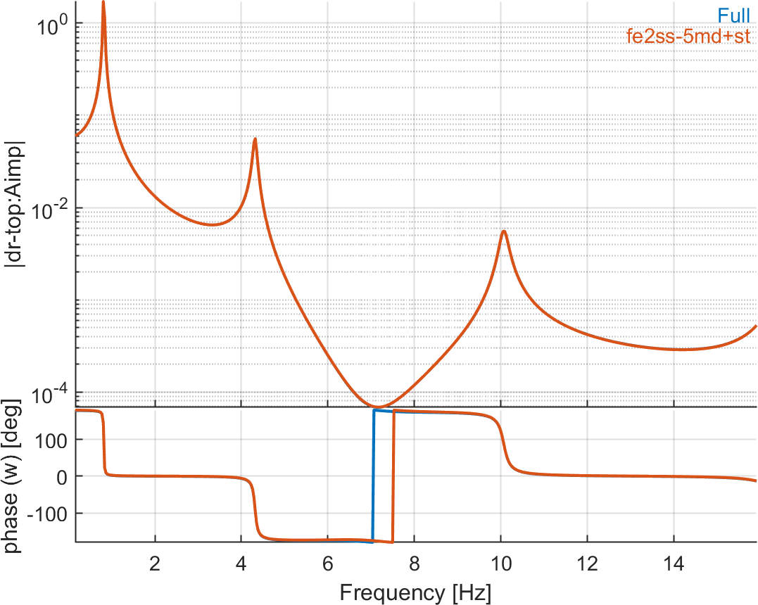
| Figure 6.7: comparison between the response (relative displacement at the top of the tower divided by imposed acceleration) of the full model computed in the frequency domain, and of the reduced state-space model using 5 modes and a static correction (dr,top/Aimp) |
In d_piezo('TutoPzTowerSSAimp-s4')
, the approach used in SDT to build a state-space model allowing to obtain directly the absolute displacement is illustrated.
TR2 = fe2ss('craigbampton 5 5 -basis',model);
sysu= nor2ss(TR2,model) ;
Figure 6.8 shows that the state-space model obtained with this approach in SDT gives a response very close to the full model computed in the frequency domain.
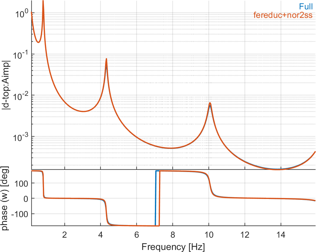
| Figure 6.8: Transfer function between horizontal acceleration at the bottom and the absolute displacement at the top of the beam and the imposed horizontal acceleration at the bottom - comparison of the full model (freq domain computation) and the reduced state-space model with 5 modes and static correction (dtop/Aimp) |
6.3.3 Model reduction and state-space models for piezoelectric structures
When building reduced or state-space models to allow faster simulation, the validity of the reduction is based on assumptions on bandwidth, which drive modal truncation, and considered loads which lead to static correction vectors.
Modes of interest are associated with boundary conditions in the absence of excitation. When using piezoelectric actuators driven in voltage mode, for the electric part, these are given by potential set to zero (grounded or shorted electrodes) and enforced by actuators (defined as DofSet in SDT in the case of voltage actuators) which in the absence of excitation is the same as shorting.
Excitation can be mechanical {Fmech}, charge on free electric potential DOF {Q}In and imposed voltage {V}In. One thus seeks to solve a problem of the form
The imposed voltage {V}In is enforced using a DofSet in SDT and is therefore analogous to an imposed displacement. The general form of the loads given above can be simplified due to the fact that there are no coupling terms in the mass matrix between the mechanical and electrical DOFs for full models of piezoelectric structures (see (6)), and the fact that the capacitance matrix [KVV] is diagonal. The problem is then reduced to
Using the classical modal synthesis approach (implemented as fe2ss('free')), one builds a Ritz basis combining modes with grounded electrodes (VIn=0), static responses to mechanical and charge loads and static response to enforced potential:
In this basis, one notes that the static response associated with enforced potential VIn does not verify the boundary condition of interest for the state-space model where VIn=0. Since it is desirable to retain the modes with this boundary condition as the first vectors of basis (41) and to include static correction as additional vectors, the strategy used here is to rewrite reduction as
where the response associated with reduced DOFs qR verifies VIn=0 and the total response is found by adding the enforced potential on the voltage DOF only. The presence of this contribution corresponds to a d term in state-space models. The usual SDT default is to include it as a residual vector as shown in (41), but to retain the shorted boundary conditions, form (42) is prefered.
6.3.4 Example of a cantilever beam with 4 piezoelectric patches
The example of the cantilever beam with 4 piezoelectric transducers detailed in section 4.6.2 is considered again. A state-space model is built using the first 10 modes and static corrections discussed above, and the dynamic response is compared to the full-model response.
In d_piezo('TutoPzPlate4pztSS-s1')
, the model is built and the actuators and sensors defined.
Then in d_piezo('TutoPzPlate4pztSS-s2')
, the transfer functions between 'V-Act', defined on the first piezoelectric patch, and , 'Q-Act', 'QS1-3', defined as charge sensors on patches 1 to 4, as well as 'Tip' (tip displacement) are computed using the full model with fesimul and the reduced state-space model built with fe2ss.
Figures 6.9 and 6.10 show that there is an excellent match between the responses computed with the full model and the state-space model with 10 modes and static corrections.
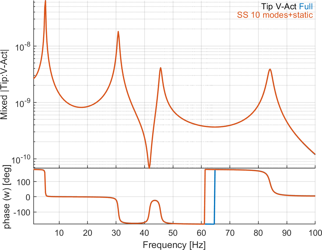
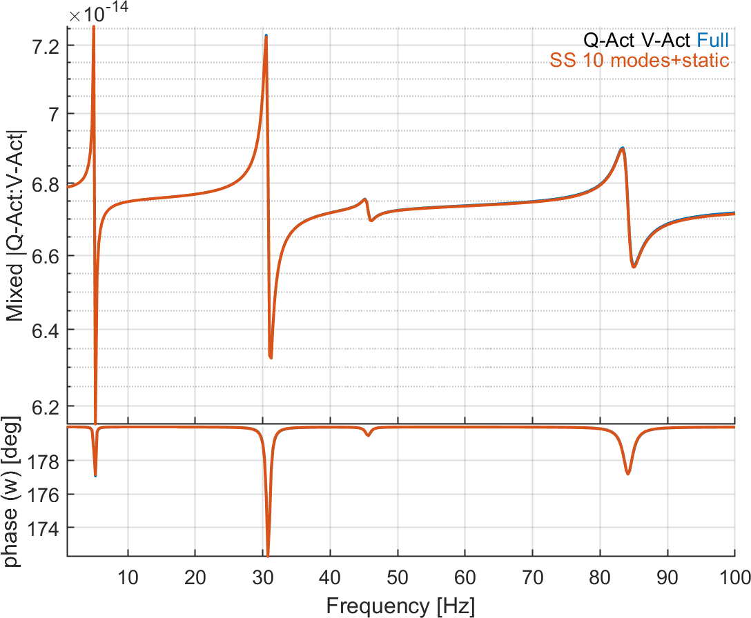
| Figure 6.9: Open-loop transfer function between V-Act and tip displacement (left), Q-Act sensor (right), comparison between, full model and reduced state-space model (10 modes + static corrections - dterm) |
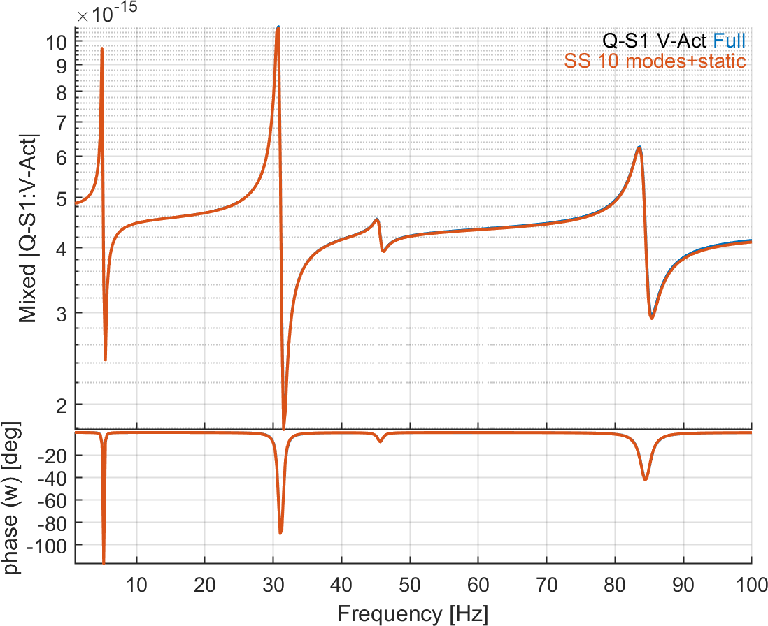
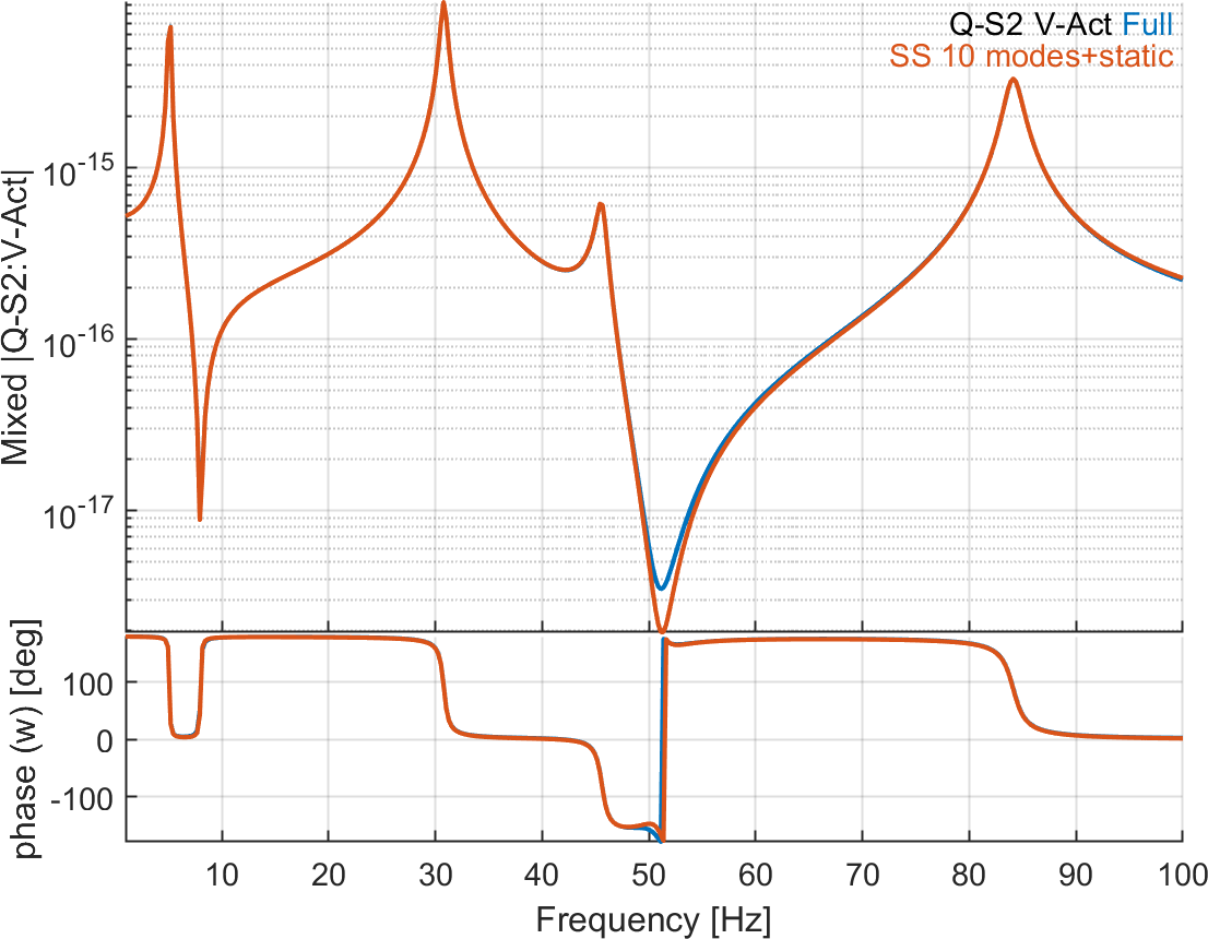
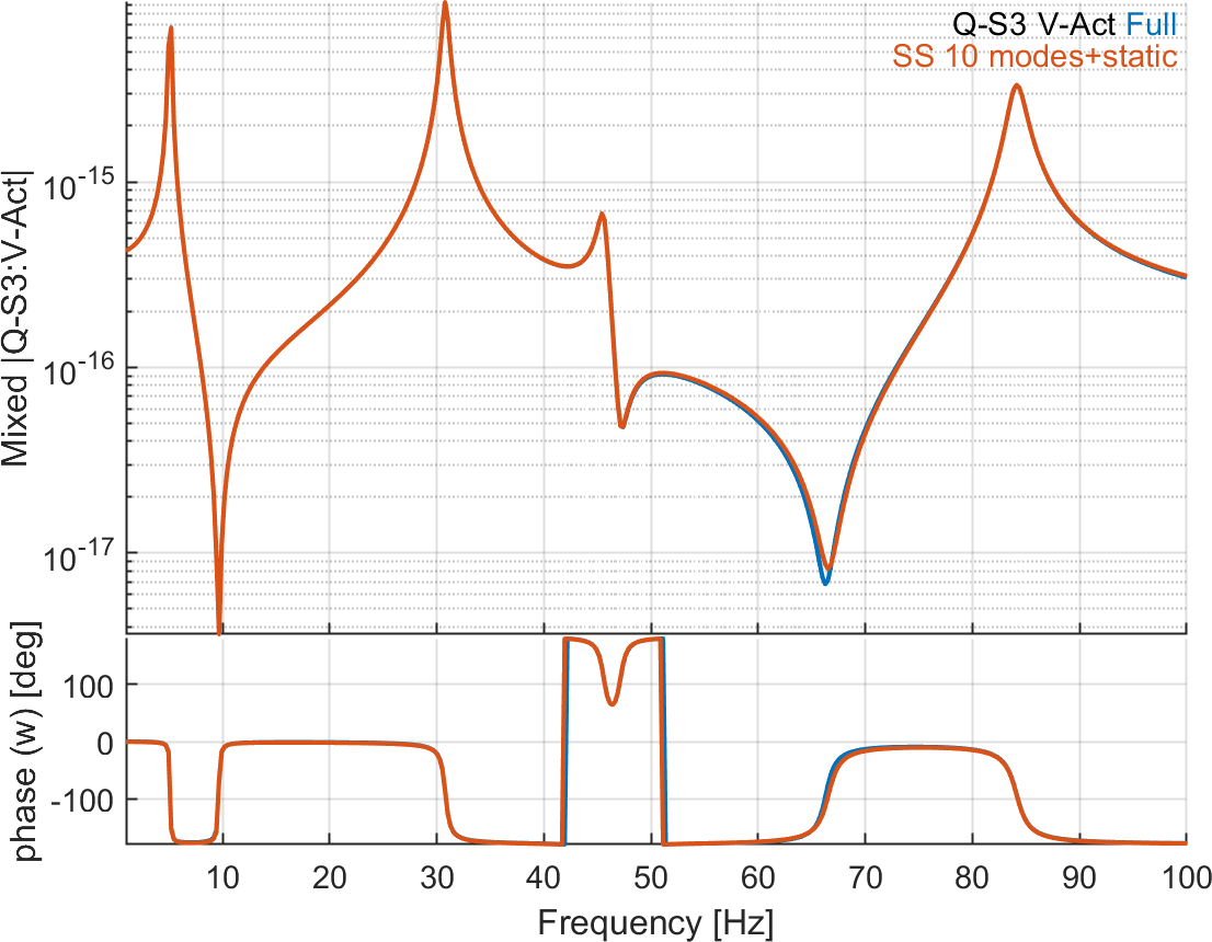
| Figure 6.10: Open-loop transfer function between V-Act and Q-S1 sensor (top-left),Q-S2 sensor (top-right), Q-S3 sensor (bottom), comparison between, full model and reduced state-space model (10 modes + static corrections - dterm) |
In the next script, we illustrate the use of sensors and actuators combinations.
In d_piezo('TutoPzPlate4pztSSComb-s1')
, we build the mesh and define actuator combinations: the first and second patch are actuated together with an opposite voltage to induce pure bending, and the static response is computed (Figure 6.11).
Then in d_piezo('TutoPzPlate4pztSSComb-s2')
, we define two sensors, consisting in charge combination with opposite signs for nodes 1057 and 1058
and voltage combination with opposite signs for the same nodes (Figure 6.12 shows the case of charge combination).
.png)
| Figure 6.11: Static deflection due to combination of actuators to induce pure bending |
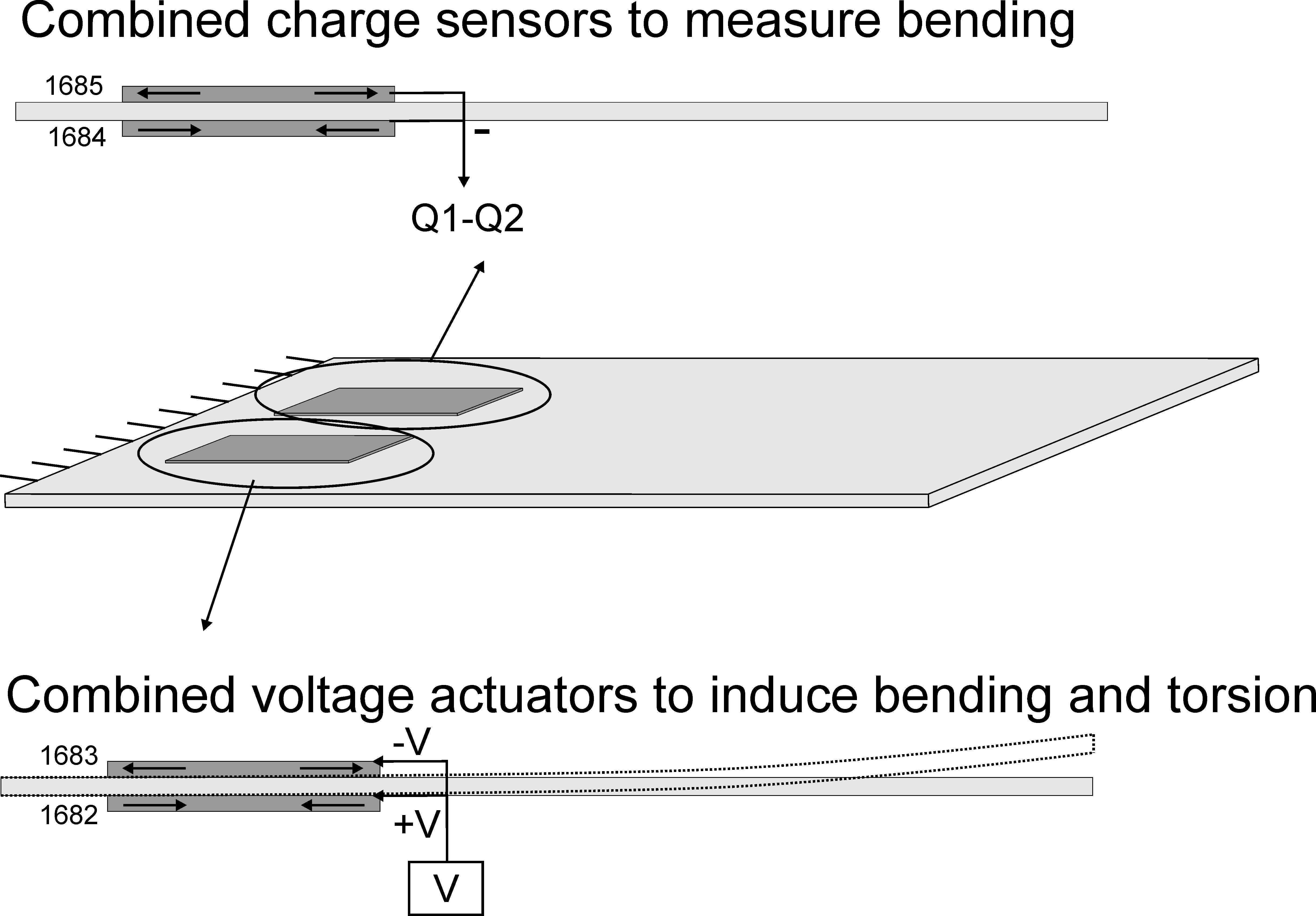
| Figure 6.12: Example of combination of charge sensors and voltage actuators to measure bending |
r1=struct('cta',[1 -1],'DOF',edofs(3:4),'name','QS3+4');
model=p_piezo('ElectrodeSensQ',model,r1);
r1=struct('cta',[1 -1],'DOF',edofs(3:4),'name','VS3+4');
model=fe_case(model,'SensDof',r1.name,r1);
model=fe_case(model,'pcond','Piezo','d_piezo(''Pcond 1e8'')');
By default, the electrodes are in 'open-circuit' condition for sensors, except if the sensor is also used as voltage
actuator which corresponds to a 'short-circuit' condition. Therefore, as the voltage is left 'free' on nodes 1057 and 1058,
the charge is zero and the combination will also be zero. If we wish to use the patches as charge sensors, we need to
short-circuit the electrodes, which will result in a zero voltage and in a measurable charge.
This is illustrated in d_piezo('TutoPzPlate4pztSSComb-s3')
by
computing the response in both configurations (open-circuit by default, and short-circuiting the electrodes for nodes 1057 and
1058):
The FRF for the combination of charge sensors is not exactly zero but has a negligible value in the 'open-circuit' condition, while the voltage
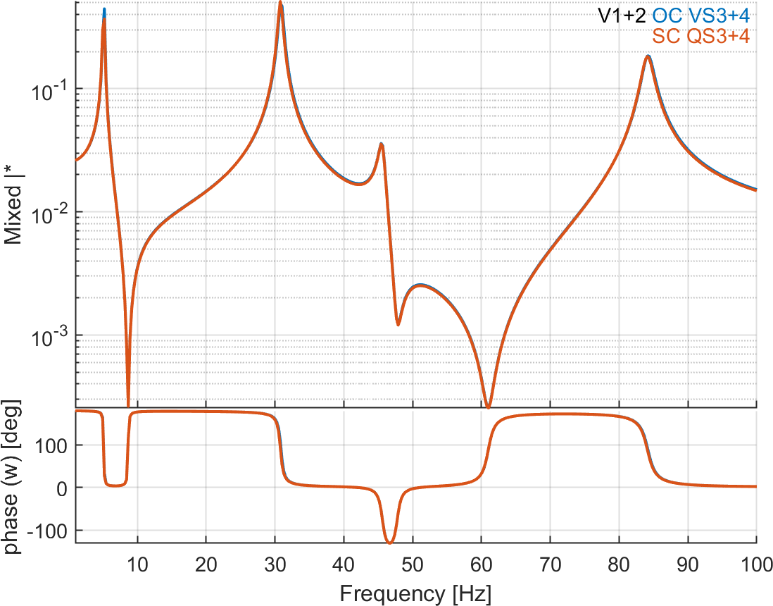
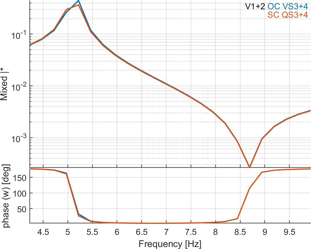
combination is equal to zero in the 'short-circuit' condition. Charge sensing in the short-circuit condition and voltage sensing in the open-circuit condition are compared by scaling the two FRFs to the static response (f=0 Hz) and the result is shown on Figure 6.13. The FRFs are very similar but the eigenfrequencies are slightly lower in the case of charge sensing. This is due to the well-known fact that open-circuit always
leads to a stiffening of the piezoelectric material. The effect on the natural frequency is however not very strong due to the small size of the piezoelectric patches with respect to the full plate.
| Figure 6.13: Comparison of FRFs (scaled to the static response) for voltage (green) and charge (blue) sensing. Zoom on the third eigenfrequency (right) |
The stiffening effect due to the presence of an electric field in the piezoelectric material when the electrodes are in the open-circuit condition is a consequence of the piezoelectric coupling. One can look at the level of this piezoelectric coupling by comparing the modal frequencies with the electrodes in open and short-circuit conditions.
This is done in d_piezo('TutoPzPlate4pztSSComb-s5')
model=d_piezo('MeshULBplate -cantilever');
d1=fe_eig(model,[5 20 1e3]);
DOF=p_piezo('electrodeDOF.*',model);
d2=fe_eig(fe_case(model,'FixDof','SC',DOF),[5 20 1e3]);
r1=[d1.data(1:end)./d2.data(1:end)];
gf=figure;plot(r1,'*','linewidth',2);axis tight; set(gca,'Fontsize',15)
xlabel('Mode number');ylabel('f_{OC}/f_{SC}');
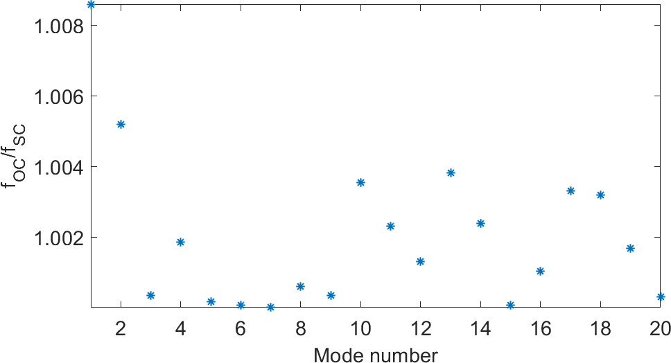
Figure 6.14 shows the ratio of the eigenfrequencies in the open-circuit vs short-circuited conditions. The difference depends
on the mode number but is always lower than 1%. Higher stiffening effects occur when more of the strain energy is contained in the piezoelectric elements, and the coupling factor is higher.
| Figure 6.14: Ratio of the natural frequencies of modes 1 to 20 in open-circuit vs short-circuit conditions illustrating the stiffening of the piezoelectric material in the open-circuit condition |
©1991-2025 by SDTools