PDF Index
| SDT-piezo
Contents
Functions
PDF Index |
For coupled problems linked to model substructuring, it is traditional to state the problem in terms of imposed displacements rather than loads. Assuming that the imposed displacements correspond to DOFs, one seeks solutions of problems of the form
| (43) |
where the displacement qI are given and the reaction forces RI are non-zero. The exact response to an imposed harmonic displacement qI is given by
| (44) |
The first level of approximation is to use a quasistatic evaluation of this response , that is to use Z(0)=[K]. Model reduction on this basis is known as static or Guyan condensation [].
This reduction does not fulfill the requirement of validity over a given frequency range. Craig and Bampton [] thus complemented the static reduction basis by fixed interface modes : normal modes of the structure with the imposed boundary condition qI=0. These modes correspond to singularities in ZCC so their inclusion in the reduction basis allows a direct control of the range over which the reduced model gives a good approximation of the dynamic response.
The Craig-Bampton reduction basis takes the special form
| (45) |
where the fact that the additional fixed interface modes have zero components on the interface DOFs is very useful to allow direct coupling of various component models. fe_reduc provides a solver that directly computes the Craig-Bampton reduction basis.
A major reason of the popularity of the Craig-Bampton (CB) reduction basis is the fact that the interface DOFs qI appear explicitly in the generalized DOF vector qR, and is a major reason why the use of Craig-Bampton reduction methods is very popular in the industry.
The major finite elements softwares such as Nastran, Abaqus or Ansys all propose a CB reduction. In the industry, it is a common practice to share models via CB reduced matrices, therefore keeping the details of the geometry and material properties confidential. Generally, the degrees of freedom which are kept in the model are the essential ones, i.e. the ones where forces are applied, or where the magnitude of displacement, velocity or acceleration needs to be assessed, as well as interface degrees of freedom if the structure needs to be coupled to one or several others. The question we address in the next section is how to build an accurate state-space model based on these reduced matrices only.
As detailed in section 6.3.1, when dealing with a full FE model, the imposed displacement can be replaced by a force equal to −[TC] [K] [TI] {qI}, neglecting the term related to acceleration. It turns out that this assumption is not valid after a CB reduction.
It can be easily understood if we consider that only the imposed degrees of freedom are retained in the CB basis. In that case, [TC] [K] [TI]=[KCI] which, according to (28) is equal to zero, would result in no load applied to the system. In this specific case, the inertial term is the most important one, while the stiffness term is zero, hence it is not possible to build a state-space model based on the standard approach presented before.
In  d_piezo('TutoPzTowerSSUimpCB-s1')
, we use low level calls to make an explicit computation of the response after CB reduction, using either the inertia, the stiffness of both terms for the loading.
d_piezo('TutoPzTowerSSUimpCB-s1')
, we use low level calls to make an explicit computation of the response after CB reduction, using either the inertia, the stiffness of both terms for the loading.
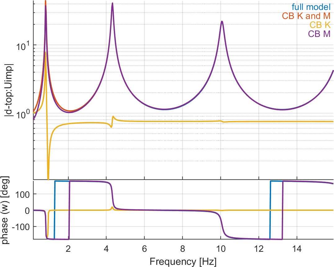
% See full example as MATLAB code in d_piezo('ScriptTutoPzTowerSSUimpCB')
d_piezo('DefineStyles');

%% Step 1 : Build Model, CB reduction, explicit response
model=d_piezo('meshtower');
model=fe_case(model,'FixDof','Clamped',[1.06]); % Leave x free for imposed displ
model=fe_case(model,'Remove','F-top'); % Remove point force
model=fe_case(model,'DOFSet','UImp',[1.01]); % Set imposed displ

%Full model matrices
[model,Case] = fe_case('assemble NoT -matdes 2 1 Case -SE',model) ;
K0 = feutilb('tkt',Case.T,model.K); % Full-model

% CB matrices and T matrix
CB    = fe_reduc('craigbampton 5 5',model); TR = CB.TR; KCB=CB.K;

% Build loads full and reduced models
F = -Case.T'*model.K{2}*Case.TIn;
F1=-CB.K{2}(2:end,1);
F2=-CB.K{1}(2:end,1);

w=linspace(1,100,512);

for i=1:length(w)
 U0(:,i)=Case.T*((K0{2}*(1+0.02*1i)-w(i)^2*K0{1})\F); % full model
 U1r(:,i)=((KCB{2}(2:end,2:end)*(1+0.02*1i)-w(i)^2*KCB{1}(2:end,2:end)) ...
  \(F1-w(i)^2*F2)); % CB stiffness and inertia
 U2r(:,i)=((KCB{2}(2:end,2:end)*(1+0.02*1i)-w(i)^2*KCB{1}(2:end,2:end)) ...
    \(F1)); % CB stiffness
 U3r(:,i)=((KCB{2}(2:end,2:end)*(1+0.02*1i)-w(i)^2*KCB{1}(2:end,2:end))...
    \(-w(i)^2*F2)); %CB inertia
end

CTA = fe_c(model.DOF,21.01); u0 = CTA*U0;
U1=TR.def*[ones(1,length(w)); U1r]; u1 = CTA*U1;
U2=TR.def*[ones(1,length(w)); U2r]; u2 = CTA*U2;
U3=TR.def*[ones(1,length(w)); U3r]; u3 = CTA*U3;

% Change output format to be compatible with iicom
C1=d_piezo('BuildC1',w'/(2*pi),u0.','d-top','Uimp'); C1.name='full model';
C2=d_piezo('BuildC1',w'/(2*pi),u1.','d-top','Uimp'); C2.name='CB K and M';
C3=d_piezo('BuildC1',w'/(2*pi),u2.','d-top','Uimp'); C3.name='CB K';
C4=d_piezo('BuildC1',w'/(2*pi),u3.','d-top','Uimp'); C4.name='CB M';
ci=iiplot;iicom(ci,'curveinit',{'curve',C1.name,C1;'curve',C2.name,C2; ...
 'curve',C3.name,C3;'curve',C4.name,C4});
iicom('submagpha')
d_piezo('setstyle',ci);
Figure 6.15 illustrates clearly the fact that the forcing term related to acceleration is the most important one to represent the response.
In practice however, the DOFs retained with Craig-Bampton are not limited to the imposed displacements. As an illustrative example, we consider that the translation DOF at the top of the tower is also kept in the CB reduction.
In d_piezo('TutoPzTowerSSUimpCB-s2')
, based on these reduced matrices, a state-space model is built with fe2ss and the response is compared to the full model.
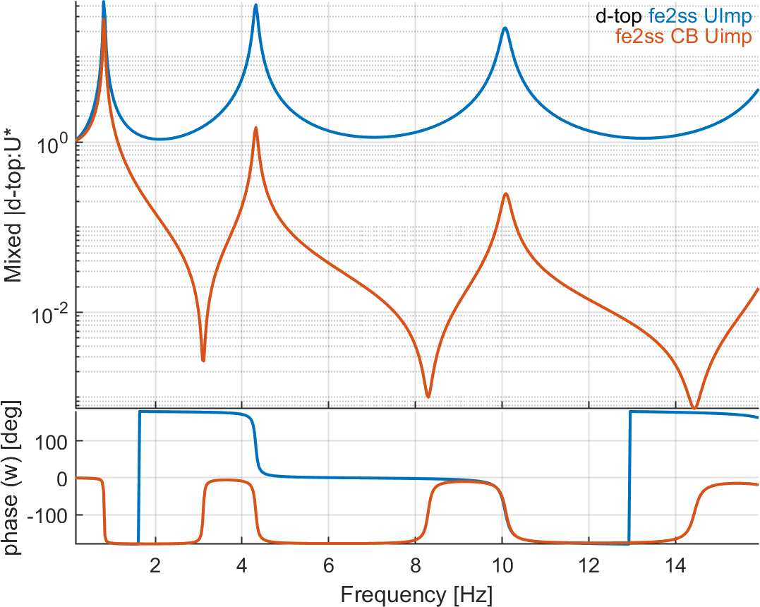
%% Step 2: keep bottom and top translation in the CB basis

% Ss from full model - 5 modes + static
sys0=fe2ss('free 5 5 0 -dterm',model);
C0=qbode(sys0,w,'struct-lab');C0.name='fe2ss'; C0.X{2}={'d-top'}

% Top and bottom DOF to be kept in CB reduction
SET.DOF=[1.01; 21.01]; SET.def=eye(2);
model=fe_case(model,'DOFSet','UImp',SET);

% Build CB reduced model
model = stack_set(model,'info','EigOpt',[5 5 0]);
SE1= fe_reduc('CraigBampton -SE -matdes 2 1 3 4 ',model); %
% To keep only the matrices
SE1 = rmfield(SE1,{'il','pl','Stack','TR','mdof'}) ;
SE1.Node=feutil('getnode',SE1,unique(fix(SE1.DOF)));SE1.Elt=[];

% Define input/output
SE1=fe_case(SE1,'SensDOF','d-top',21.01);
SE1=fe_case(SE1,'DOFSet','UImp',[1.01]); %

% Build state-space based on CB reduced model
sys=fe2ss('free 5 5 0 -dterm',SE1);
Figure 6.16 shows that using fe2ss after a CB reduction leads to a very bad reduced state-space representation of the dynamics of the beam with imposed displacement.
An alternative is to use a transformation of the CB mass and stiffness matrices in order to come back to a situation where the inertial term in the excitation is zero, and only the stiffness term is non-zero, so that fe2ss can be applied to build the state-space model. The transformation is applied so that the retained DOFs are untouched (so that they represent physical DOFs and can be used to simply apply force and measure output quantities), as proposed in []. Raze's transform takes the form:
| (46) |
Therefore the matrices can be transformed with the following projection matrix
| (47) |
It is straightforwardd to show that after applying the transformation, matrix [M_CI]=0, so that now only the stiffness term appears in the excitation term. After transforming the matrices, fe2ss can be used to build an accurate reduced state-space model.
In In d_piezo('TutoPzTowerSSUimpCB-s3')
, we first perform the transformation manually with low-level calls and replace the matrices in the reduced model, then we use the '-noMCI' option in fe_reduc which allows to apply the CB reduction and Raze's transform in one step.
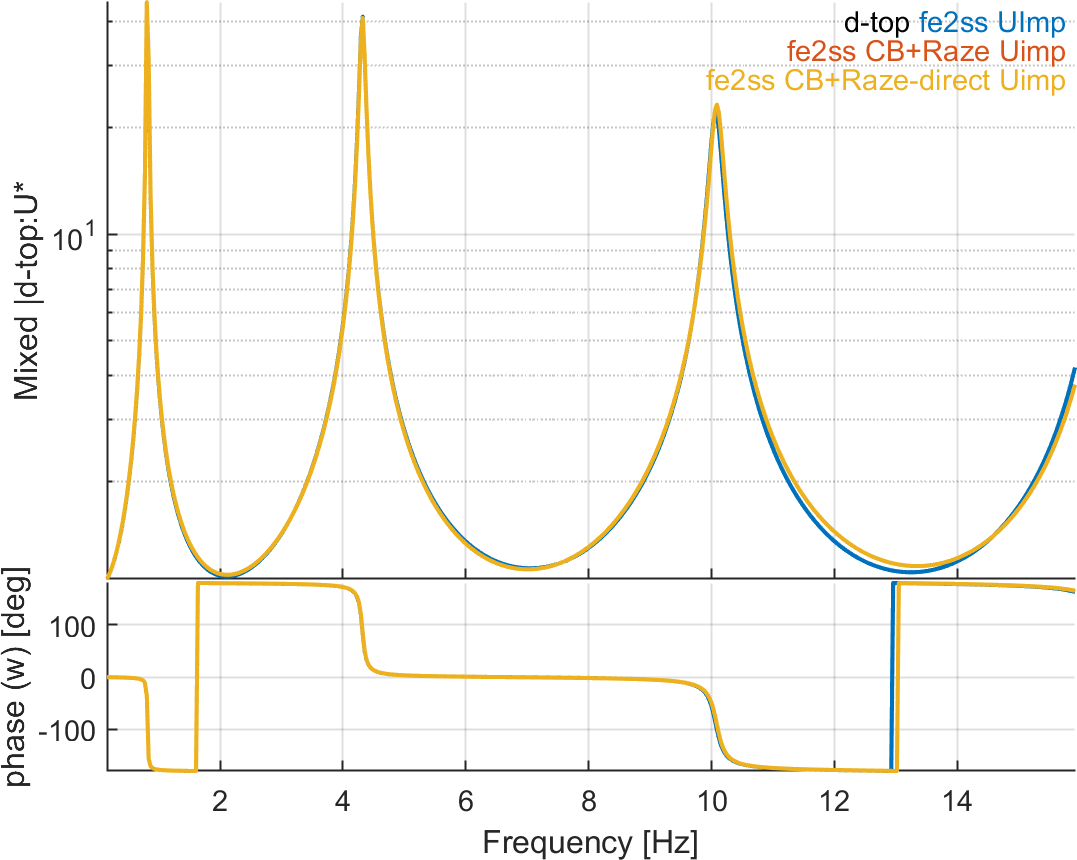
%% Step 3 : Apply Raze transform before making the state-space model

% Transform the initial CB matrices
KCB=SE1.K;
N=size(KCB{1},1);
T1=[ eye(2) zeros(2,N-2) ; - KCB{1}(3:end,3:end)\KCB{1}(3:end,1:2) eye(N-2)];

Mr=T1'*(KCB{1})*T1;
Kr=T1'*(KCB{2})*T1;

% Replace matrices in the CB model
SE2=SE1;
SE2.K{1}=Mr;
SE2.K{2}=Kr;

sys2=fe2ss('free 5 5 0 -dterm',SE2);

% Make CB matrices with Raze's transform directly -noMCI
SE3= fe_reduc('CraigBampton -SE -matdes 2 1 3 4 -noMCI',model);

% To keep only the matrices
SE3 = rmfield(SE3,{'il','pl','Stack','TR','mdof'}) ;
SE3.Node=feutil('getnode',SE3,unique(fix(SE3.DOF)));SE3.Elt=[];

% Define input/output
SE3=fe_case(SE3,'SensDOF','d-top',21.01);
SE3=fe_case(SE3,'DOFSet','UImp',[1.01]); %

% Build state-space based on CB reduced model
sys3=fe2ss('free 5 5 0 -dterm',SE3);
Figure 6.17 shows that using fe2ss after a CB and Raze's transformation given by (47) leads to an accurate model in the frequency band of interest
The case of imposed acceleration is much simpler to treat as fe2ss can be used directly after CB reduction in the case of relative displacement. If one is interested in absolute displacement, nor2ss can be applied after computing the modeshapes based on the reduced CB matrices and having orthonormalized them. The first script illustrates the construction of a state-space model for relative displacement, using fe2ss and the definition of an equivalent load.
In d_piezo('TutoPzTowerSSAimpCB-s1')
, the reference solution is computed using explicit computations with low-level calls.
Then in d_piezo('TutoPzTowerSSAimpCB-s2')
, a CB reduction is performed keeping the displacement in the x-direction for the nodes at the bottom and at the top of the tower and 5 modes.
%% Step 1: reference solution -direct computation

% Build model
model=d_piezo('meshtower');
model=fe_case(model,'FixDof','Clamped',[1.06]);
% Leave x free for imposed displ
model=fe_case(model,'Remove','F-top'); % Remove point force

% Initial matrices without imposed displacements
[model0,Case0] = fe_case('assemble NoT -matdes 2 1 Case -SE',model) ;
K0 = feutilb('tkt',Case0.T,model0.K); % Full-model 41x41

% Matrices with Block displ at basis
model=fe_case(model,'DOFSet','UImp',[1.01]); %

% Full model matrices
[model,Case] = fe_case('assemble NoT -matdes 2 1 Case -SE',model) ;
Kcc = feutilb('tkt',Case.T,model.K); % Blocked at basis 40x40

% Put manually unitary values to be exact
TIn=zeros(40,1); TIn(1:2:end)=1;

% The load is built after applying the boundary condition to the matrices.
F = -(Kcc{1}*TIn);

w=linspace(0,100,512);
eta=0.02;

% Reference solution - full model
for i=1:length(w)
    U0(:,i)=Case.T*((Kcc{2}*(1+eta*1i)-w(i)^2*Kcc{1})\F);
end

CTA = fe_c(model.DOF,21.01); u0 = CTA*U0;
% Change output format to be compatible with iicom
C0=d_piezo('BuildC1',w'/(2*pi),u0.','dr-top','Aimp'); C0.name='Full';
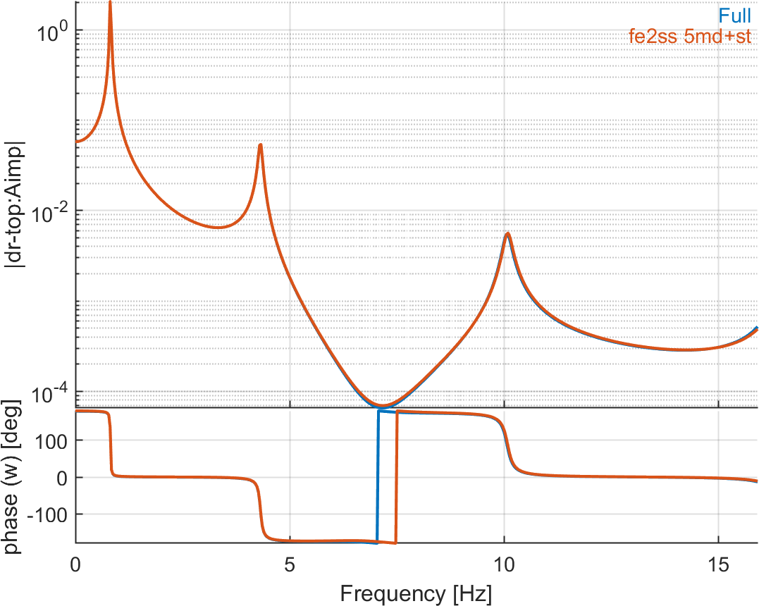
%% Step 2 : state-space model based on CB reduction

% CB reduction on two DOFs
SET.DOF=[1.01; 21.01]; SET.def=eye(2);
model=fe_case(model,'DOFSet','UImp',SET);

% Build CB reduced model
model = stack_set(model,'info','EigOpt',[5 5 0]); % No mass shift!
SE1= fe_reduc('CraigBampton -SE -matdes 2 1 3 4 -bset ',model); %

SE0=SE1; % Save superelement model

% To keep only the matrices
SE1 = rmfield(SE1,{'il','pl','Stack','TR','mdof'}) ;
SE1.Node=feutil('getnode',SE1,unique(fix(SE1.DOF)));SE1.Elt=[];

% Force vector using CB matrices
KCB=SE1.K;
TInCB= [1; -KCB{2}(2:end,2:end)\KCB{2}(2:end,1)];
FCB= -KCB{1}*TInCB; % From CB matrices only


% Block 1.01 and define a DofLoad and a new observation matrix instead
SE1=fe_case(SE1,'FixDOF','BC',1.01); % BC for relative displacement
SET.DOF=SE1.DOF(2:end); SET.def= FCB(2:end);
SE1=fe_case(SE1,'DOFLoad','UImp',SET); % Equivalent load
SE1=fe_case(SE1,'SensDOF','Output',SET.DOF(1));

sys=fe2ss('free 5 5 0 -dterm',SE1);
Figure 6.18 shows that using fe2ss with applied load leads to an accurate model in the frequency band of interest
In d_piezo('TutoPzTowerSSAimpCB-s3')
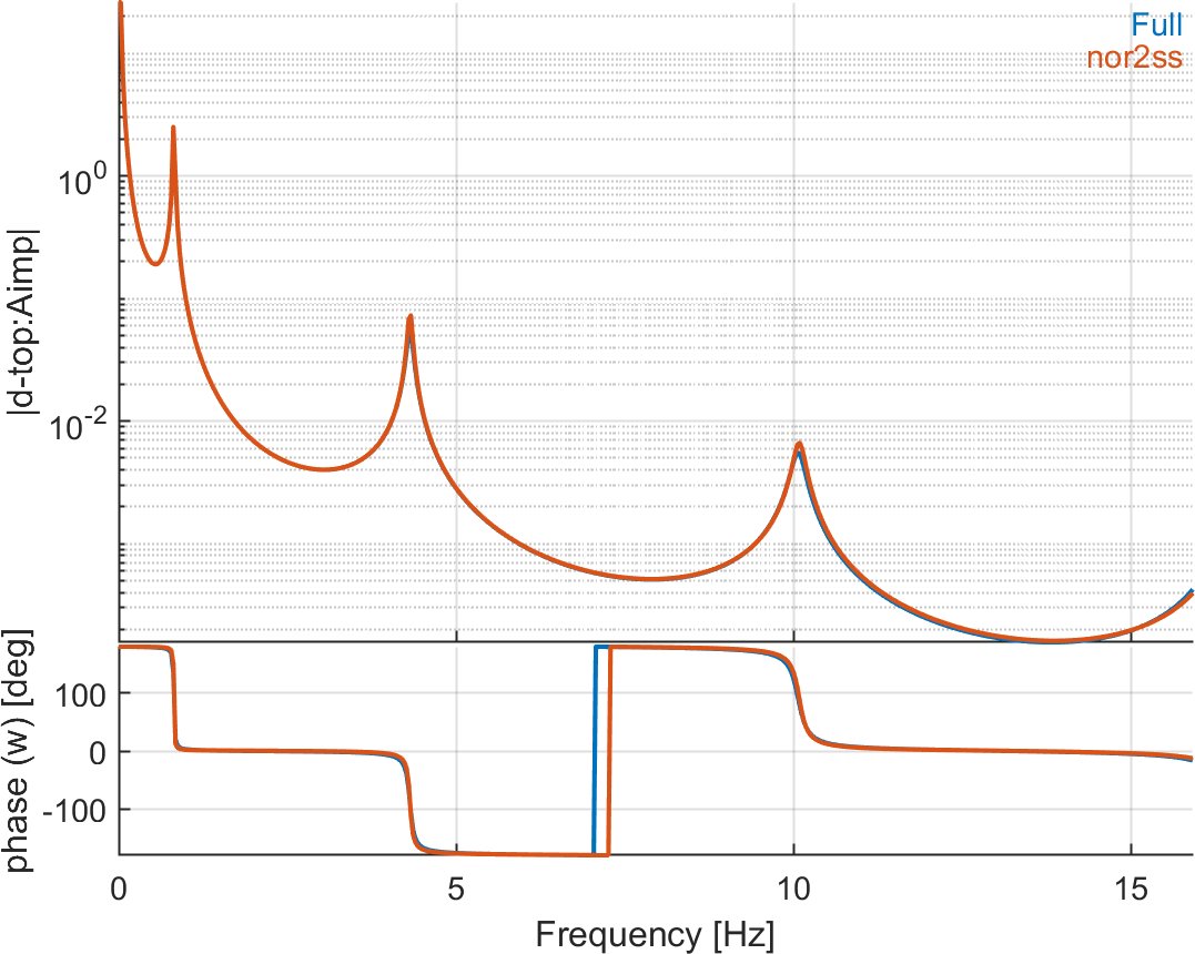
, the state-space model with an output in absolute displacements is built using nor2ss and the response iscompared to the reference solution.
%% Step 3: State-space model with absolute displacement

SE2=SE0; % Initial model without BCs
TR2=fe_eig(SE2,[5 7 0]); % Compute all7  modes of reduced model

% Imposed acceleration at base
SET.DOF=[1.01]; SET.def=eye(1); %
SE2=fe_case(SE2,'DOFSet','UImp',SET); % Impose acc at bottom

% build state-space model with nor2ss
sys2= nor2ss(TR2,SE2) ;
Figure 6.19 shows that using nor2ss with imposed acceleration leads to an accurate model in the frequency band of interest
We are considering again the aluminum plate with 4 piezoelectric patches shown in Figure 4.19 and with the material properties in Table 4.1.
In d_piezo('TutoPzPlate4pztSSCB-s1')
, a reference state-space model is first built with fe2ss using 5 modes in the reduced basis and the static correction linked to the voltage actuator.
In d_piezo('TutoPzPlate4pztSSCB-s2')
, a Craig-Bampton model reduction is performed choosing the 4 electrical DOFs corresponding to each patch and the displacement sensor at the tip of the beam as reference DOFs. The reduced matrices are used to build a super-element, and the response is computed as for the reference using directly fe2ss.
Figure 6.20 shows the errors introduced due to the fact that there is a mass coupling term after CB.
%% Step 2 - CB reduction
model=fe_case(model,'DOFSet','In',[nd+.03; i1+.21]); %

% Build CB matrices
model = stack_set(model,'info','EigOpt',[5 10 0]);
SE1= fe_reduc('CraigBampton -SE -matdes 2 1 3 4 -bset',model); %
% To keep only the matrices
SE1 = rmfield(SE1,{'il','pl','Stack','TR'}) ;
SE1.Node=feutil('getnode',SE1,unique(fix(SE1.DOF)));SE1.Elt=[];

% Define node names
SE1=sdth.urn('nmap.Node.set',SE1, ...
    {'Tip',nd;'Act',i1(1);'S1',i1(2);'S2',i1(3);'S3',i1(4)});

% Define input/output
SE1=fe_case(SE1,'SensDof','Sensors',scell);
SE1=fe_case(SE1,'DofSet','In',rmfield(dIn,'Elt')); % Elt defined for display
SE1=stack_set(SE1,'info','DefaultZeta',1e-2);

% Build state-space model based on reduced CB matrices
s1=fe2ss('free 5 10 0 -dterm',SE1);
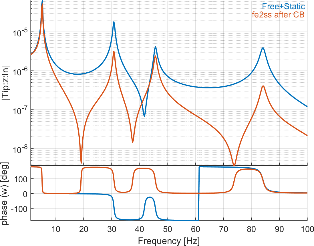
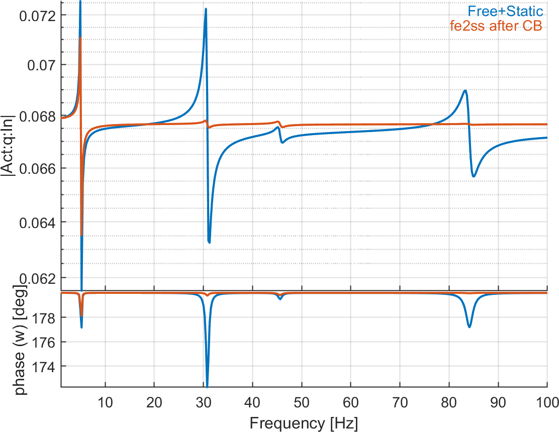
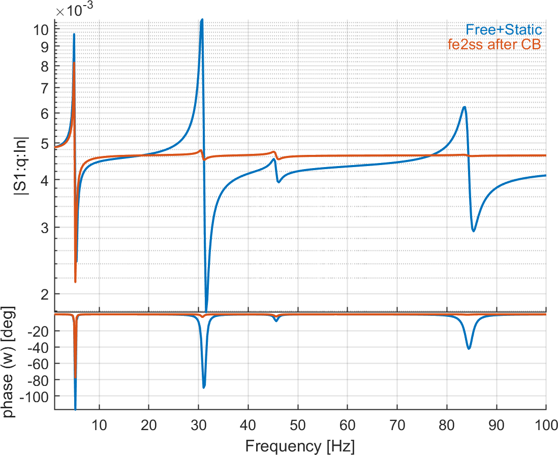
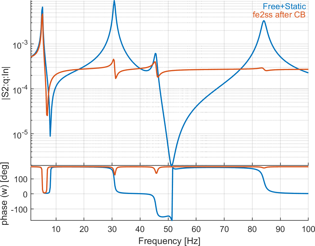
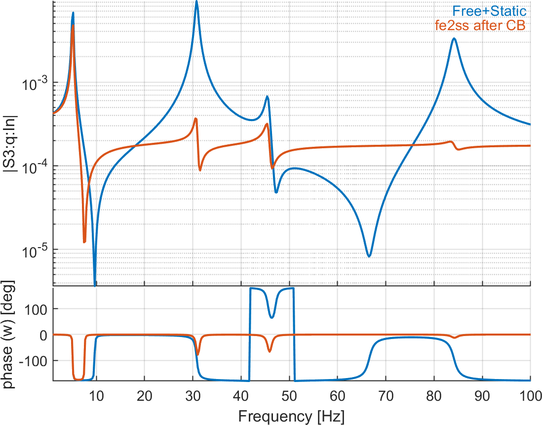
Figure 6.20: Tip displacement and charges on the 4 patches due to voltage actuator on patch 1. The reference solution is computed with a direct modal reduction (10 modes) with static correction, while the second curve represents the response after using CB reduction (10 modes + 5 retained DOFs) before building the state-space model. The second curve is wrong due to the coupling in the mass matrix introduced by the CB reduction
In In d_piezo('TutoPzPlate4pztSSCB-s3')
, we use Raze's transform to remove the coupling terms in the mass matrix (-noMCI option in fe_reduc).
Figure 6.21 shows the result when making the transform to remove mass coupling term after CB. The match with the referene solution is excellent.
%% Step 3: Now with Raze's transform, using -noMCI option in fe_reduc
SE2= fe_reduc('CraigBampton -SE -matdes 2 1 3 4 -noMCI',model); % Removes M-coupling
% To keep only the matrices
SE2 = rmfield(SE2,{'il','pl','Stack','TR'}) ;
SE2.Node=feutil('getnode',SE2,unique(fix(SE2.DOF)));SE2.Elt=[];

%Define node names
SE2=sdth.urn('nmap.Node.set',SE2, ...
    {'Tip',nd;'Act',i1(1);'S1',i1(2);'S2',i1(3);'S3',i1(4)});
% Define input/output
SE2=fe_case(SE2,'SensDof','Sensors',scell);
SE2=fe_case(SE2,'DofSet','In',rmfield(dIn,'Elt')); % Elt defined for display
SE2=stack_set(SE2,'info','DefaultZeta',1e-2);

% Build state-space model based on reduced CB matrices
s2=fe2ss('free 5 10 0 -dterm',SE2);
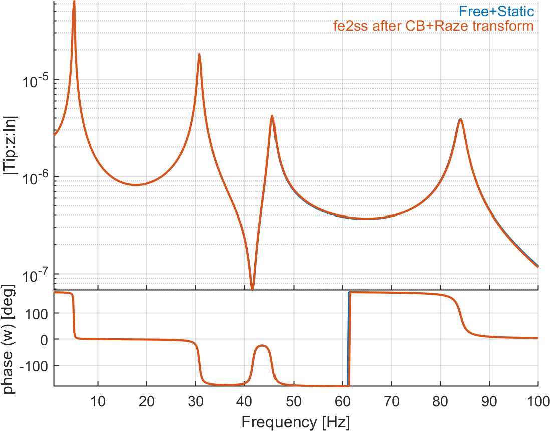
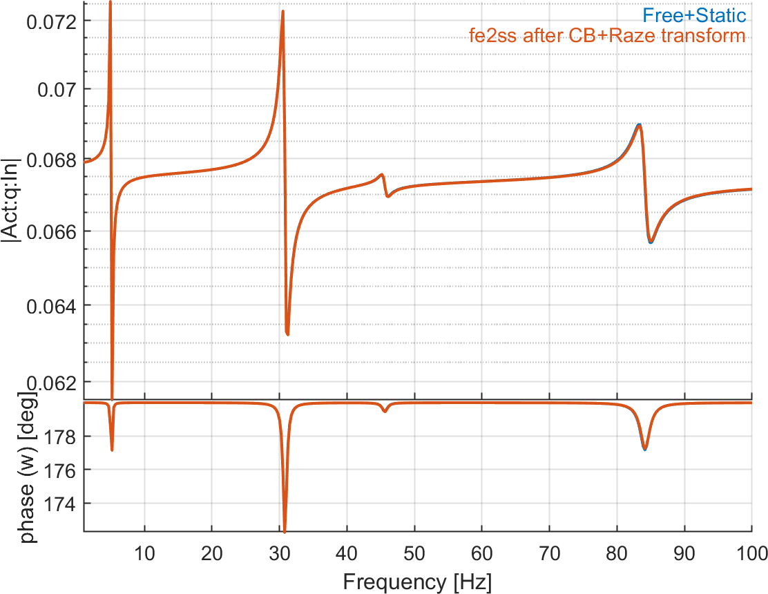
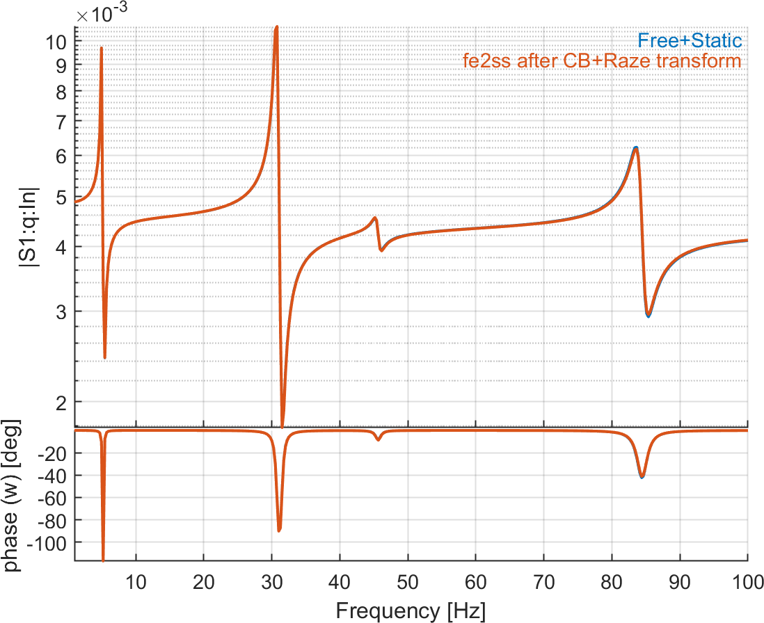
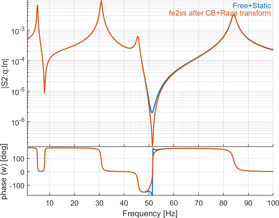
Figure 6.21: Tip displacement and charge on patches due to voltage actuator on patch 1. The reference solution is computed with a direct modal reduction (10 modes) with static correction, while the second curve represents the response after using CB reduction and Raze's transform (10 modes + 5 retained DOFs) before building the state-space model. There is an excellent match between the two curves