State space models

SDT-piezo Contents Functions

6.2 State space models

6.2.1 General theory

While normal mode models are appropriate for structures, state-space models allow the representation of more general linear dynamic systems and are commonly used in the Control Toolbox or Simulink. The standard form for state space-models is

(12)

with inputs {u}, states {x} and outputs {y}. State-space models are represented in the SDT, as generally done in other Toolboxes for use with MATLAB, using four independent matrix variables a, b, c, and d (you should also take a look at the LTI state-space object of the Control Toolbox).

The transfer functions from inputs to outputs are described in the frequency domain by

(13)

A state-space representation of the nominal structural model (1) is given by

(14)

The interest of this representation is mostly academic because it does not preserve symmetry (a useful feature of models of structures associated to the assumption of reciprocity) and because [M]⁻¹[K] is usually a full matrix (so that the associated memory requirements for a realistic finite element model would be prohibitive). The SDT thus always starts by transforming a model to the normal mode form and the associated state-space model .

The natural state-space representation of normal mode models (4) is given by

(15)

Transformations to this form are provided by nor2ss and fe2ss. Note however that, as demonstrated in section 6.1.3, using strictly the modeshapes in the reduced state-space model is generally not sufficient to obtain a proper representation of the zeros, which are very important in control applications. fe2ss uses two different representations for reduced state-space models based on normal modes and static corrections, which are detailed in the next section.

6.2.2 State-space formulations with static correction

As shown in section 6.1.2, it is possible to augment the basis of modeshapes with static corrections to applied loads to form an accurate reduction basis. Once the basis is orthonormalized, the additional vectors due to static corrections appear as additional modes in the basis. The transformation to a state-space model is straightforward using (15), but has the disadvantage to increase considerably the size of the model if a large number of input forces are considered. An alternative is presented below.
We recall that the modal decomposition of the flexibility matrix given by:

(16)

can be rewritten using (10) as:

(17)

which shows that the last two terms are proportional to the input [b] and constant (do not depend on ω). They can therefore be introduced in matrix d of the state-space model, with matrices a,b and c corresponding to the case where only the normal modes are retained (15). The state-space model then becomes :

(18)

where

(19)

The advantage of building the state-space model with such an approach is that the number of degrees of freedom is not increased, and that the [d] matrix introduces a static contribution which cannot be destabilized by a controller, if active damping is applied for example. It introduces however a non-physical feed-through term which is directly proportional to the input force. This violates the principles of wave propagation: if the response to a rectangular impulse is computed for example, the wave should arrive to the sensors after a time related to the distance and wave velocity in the medium, and here, due to the non-zero [d] matrix, a part of it arrives instantaneously.
Building state-space models with static corrections but no additional high-frequency modes can be done with the option -dterm in fe2ss.

6.2.3 State-space models with static correction: illustration on the tower example

The cantilever beam (tower) example presented in section 6.1.3 is considered again, and the two approaches (additional mode and [d] matrix approach) to build a state-space model are illustrated below.
The first step d_piezo('TutoPzTowerSS-s1') consists in building the mesh and defining actuators and sensors as before.

Then in d_piezo('TutoPzTowerSS-s2') , the state-space model is created either with a 'dterm' or with an additional mode, and the transfer function between 'F-top' and 'd-top' is computed.

% Step 2 : State-space models
[sys,TR] = fe2ss('free 5 3 0 -dterm',model);
[sys2,TR2] = fe2ss('free 5 3 0 ',model);

w=linspace(0,30*2*pi,512);% Frequency range
% Convert to curve object and relabel X (fe2ss uses dofs and not sens/act names)
C1=qbode(sys,w,'struct-lab');C1.name='SS-dterm'; C1.X{2}={'d-top'}; 
C2=qbode(sys2,w,'struct-lab');C2.name='SS-mode'; C2.X{2}={'d-top'}; 
ci=iiplot;
iicom(ci,'curveinit',{'curve',C1.name,C1;'curve',C2.name,C2}); iicom('submagpha')
d_piezo('setstyle',ci);

Figure 6.4 shows that with the two approaches, the state-space model gives a correct representation of the transfer function in the frequency band of interest [0 10] Hz, but that the behavior is different at higher frequencies. The -dterm option does not introduce a high frequency mode, but the transfer function does not have a high-frequency roll-off due to the added constant term.

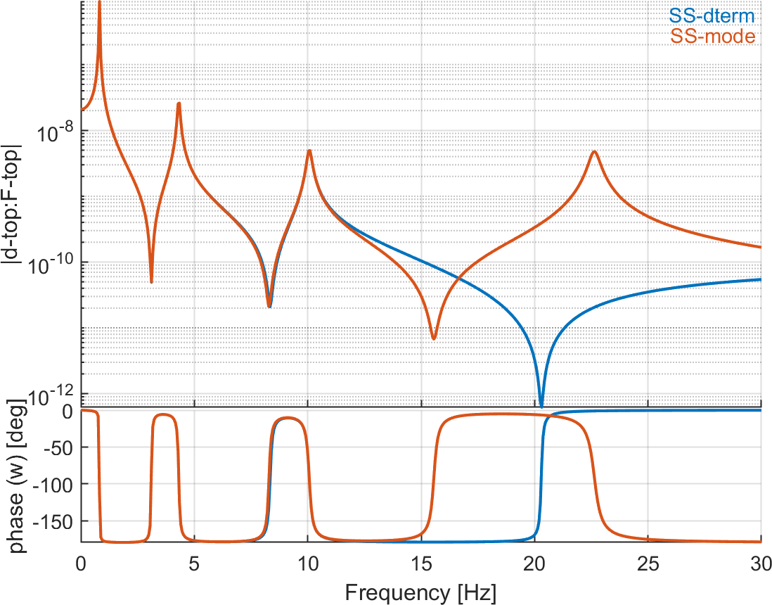
Figure 6.4: Transfer function between the tip displacement and the tip force: Comparison between state-space models using the d-term approach or the additional high-frequency mode for static correction