PDF Index
| SDT-piezo
Contents
Functions
PDF Index |
Finite element models of structures need to have many degrees of freedom to represent the geometrical details of complex structures. For models of structural dynamics, one is however interested in
These restrictions on the expected predictions allow the creation of low order models that accurately represent the dynamics of the full order model in all the considered loading/parameter conditions.
Model reduction procedures are discrete versions of Ritz/Galerkin analyzes: they seek solutions in the subspace generated by a reduction matrix T. Assuming {q} = [T] {qR}, the second order finite element model (1) is projected as follows
| (1) |
Modal analysis, model reduction, component mode synthesis, and related
methods all deal with an appropriate selection of singular projection bases
([T]N × NR with NR ≪ N). This section summarizes the theory behind these methods with references to other works that give more details.
The solutions provided by SDT make two further assumptions which are not hard limitations but allow more consistent treatments while covering all but the most exotic problems. The projection is chosen to preserve reciprocity (left multiplication by TT and not another matrix). The projection bases are assumed to be real.
An accurate model is defined by the fact that the input/output
relation is preserved for a given frequency and parameter range
| (2) |
where Z(s,α) is the dynamic flexibility Z(s)=[K+Cs+Ms2] for a given set of parameters α
Traditional modal analysis, combines normal modes and static
responses. Component mode synthesis (CMS) methods extend the
selection of boundary conditions used to compute the normal modes.
The SDT further extends the use of reduction bases to
parameterized problems.
A key property for model reduction methods is that the input/output behavior of a model only depends on the vector space generated by the projection matrix T. Thus  implies that
| (3) |
This equivalence property is central to the flexibility provided by the SDT in CMS applications (it allows the decoupling of the reduction and coupled prediction phases) and modeshape expansion methods (it allows the definition of a static/dynamic expansion on sensors that do not correspond to DOFs).
Normal modes are defined by the eigenvalue problem
| (4) |
based on inertia properties (represented by the positive definite mass matrix M) and underlying elastic properties (represented by a positive semi-definite stiffness K). The matrices being positive, there are N independent eigenvectors {φj} (forming a matrix noted [φ]) and eigenvalues ωj2 (forming a diagonal matrix noted [\ ωj2 \ ]).
As solutions of the eigenvalue problem (4), the full set of
N normal modes verify two orthogonality conditions with respect
to the mass and the stiffness
| (5) |
where µ is a diagonal matrix of modal masses
(which are quantities depending uniquely on the way the eigenvectors
φ are scaled).
In the SDT, the normal modeshapes are assumed to be mass
normalized so that [µ]= [I] (implying [φ]T [M]
[φ]=[I] and [φ]T [K] [φ] = [\ ωj2 \ ]).
The mass normalization of
modeshapes is independent from a particular choice of sensors or
actuators.
Another traditional normalization is to set a particular component of  to 1. Using an output shape matrix this is equivalent to
  (the observed motion at sensor cl is unity).
  , the modeshape with a component scaled to 1, is related to the mass normalized modeshape by
  .
.
| (6) |
is called the modal or generalized mass at sensor cl.
Modal stiffnesses are are equal to
| (7) |
The use of mass-normalized modes, simplifies the normal mode form (identity mass matrix) and allows the direct comparison of the contributions of different modes at similar sensors. From the orthogonality conditions, one can show that, for an undamped model and mass normalized modes, the dynamic response is described by a sum of modal contributions
| (8) |
which correspond to pairs of complex conjugate poles λj=± iωj.
In practice, only the first few low frequency modes are determined,
the series in (8) is truncated, and a correction for the
truncated terms is introduced (see section 6.1.2).
Normal modes are computed to obtain the spectral decomposition (8). In practice, one distinguishes modes that have a resonance in the model bandwidth and need to be kept and higher frequency modes for which one assumes ω ≪ ωj. This assumption leads to
| (9) |
For applications in reduction of finite element models, from the orthogonality conditions (5), one can easily show that for a structure with no rigid body modes (modes with ωj=0)
| (10) |
The static responses [K] −1 [b] are called attachment modes in Component Mode Synthesis applications []. The inputs [b] then correspond to unit loads at all interface nodes of a coupled problem.
One has historically often considered residual attachment modes defined by
| (11) |
where NR is the number of normal modes retained in the reduced model.
The vector spaces spanned by [φ1 … φNR TA] and [φ1 … φNR TAR] are clearly the same, so that reduced models obtained with either are dynamically equivalent. For use in the SDT, you are encouraged to find a basis of the vector space that diagonalizes the mass and stiffness matrices (normal mode form which can be easily obtained with fe_norm).
Reduction on modeshapes is sometimes called the mode displacement method, while the addition of the static correction leads to the mode acceleration method.
When reducing on these bases, the selection of retained normal modes guarantees model validity over the desired frequency band, while adding the static responses guarantees validity for the spatial content of the considered inputs. The reduction is only valid for this restricted spatial/spectral content but very accurate for solicitation that verify these restrictions.
Defining the bandwidth of interest is a standard difficulty with no definite answer. The standard, but conservative, criterion (attributed to Rubin) is to keep modes with frequencies below 1.5 times the highest input frequency of interest.
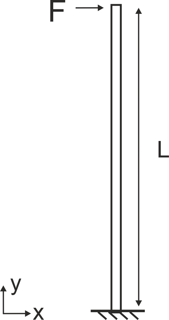
The concepts of model reduction using normal modes and static corrections are illustrated on a cantilever beam example. Figure 6.1 shows a tower of height L=140m excited at the tip and for which the displacement in the horizontal direction is computed at the same point where the excitation is applied (leading to a collocated transfer function). The full model solution is compared to a truncated solution where NR=3. The beam is made of concrete with a Young's modulus E=30GPa, a Poisson's ratio ν=0.2 and a mass density ρ=2200kg/m3. The section of the beam is a square hollow section with outer dimensions 20m x 20m and a thickness of 30cm.
The script below details explicitely the different steps to compute the response using the reduced model. It uses low-level calls which are not computationally efficient in SDT but illustrate the strategy.
The first step  d_piezo('TutoPzTowerRed-s1')
consists in building the mesh, preassembling the matrices [K] and [M] and defining the tip-load and tip-sensor.
d_piezo('TutoPzTowerRed-s1')
consists in building the mesh, preassembling the matrices [K] and [M] and defining the tip-load and tip-sensor.
The frequency band of interest is [0 10] Hz, in d_piezo('TutoPzTowerRed-s2')
, we only keep the mode shapes which have a frequency below 15 Hz (1.5 x 10 Hz), i.e. in this case the first three bending modes, and compute the transfer function between a force acting on the tip of the beam in the horizontal direction, and the displacement at the tip in the same direction. We use first explicit computations after building matrices, which is not the most efficient in terms of computational time, but is aimed at illustrating the methodology with low-level calls.
%% Step 2 : Build Reduced basis (3 modes) and compute TF

% M and K matrices have been built with fe_mknl in d_piezo('MeshTower')
M=model.K{1}; K=model.K{2};
% Excitation
Load=fe_load(model); b=Load.def;

% Projection matrix for output
sens=fe_case(model,'sens');
[Case,model.DOF]=fe_mknl('init',model); % Build Case.T for active dofs
cta=sens.cta*Case.T;

% Compute Modeshapes
def=fe_eig(model);
% Rearrange with active dofs only
def.def=Case.T'*def.def; def.DOF=Case.T'*def.DOF;

% Build reduced basis on three modes
T=def.def(:,1:3);

% Reduce matrices and compute response - explicit computation
Kr=T'*K*T; Mr=T'*M*T; br=T'*b;

% Define frequency vector for computations
w=linspace(0,30*2*pi,512);% Extended frequency range

% Solution with full and reduced matrices - explicit computation
% Use loss factor =0.02 = default for SDT (1% modal damping)
for i1=1:length(w)
    U(:,i1)=(K*(1+0.02*1i)-w(i1)^2*M)\b;
    %Default loss factor is 0.02 in SDT
    Ur(:,i1)=(Kr*(1+0.02*1i)-w(i1)^2*Mr)\br; %Reduced basis
end

% Extract response on sensor and visualize in iicom
out1=cta*U; out2=cta*(T*Ur);

% Change output format to be compatible with iicom
C0m=d_piezo('BuildC1',w'/(2*pi),out1.','d-top','F-top'); C0m.name='Full';
C1m=d_piezo('BuildC1',w'/(2*pi),out2.','d-top','F-top'); C1m.name='3md';
ci=iiplot;iicom(ci,'curveinit',{'curve',C0m.name,C0m;'curve',C1m.name,C1m});
iicom('submagpha')
d_piezo('setstyle',ci); set(gca,'XLim',[0 10])
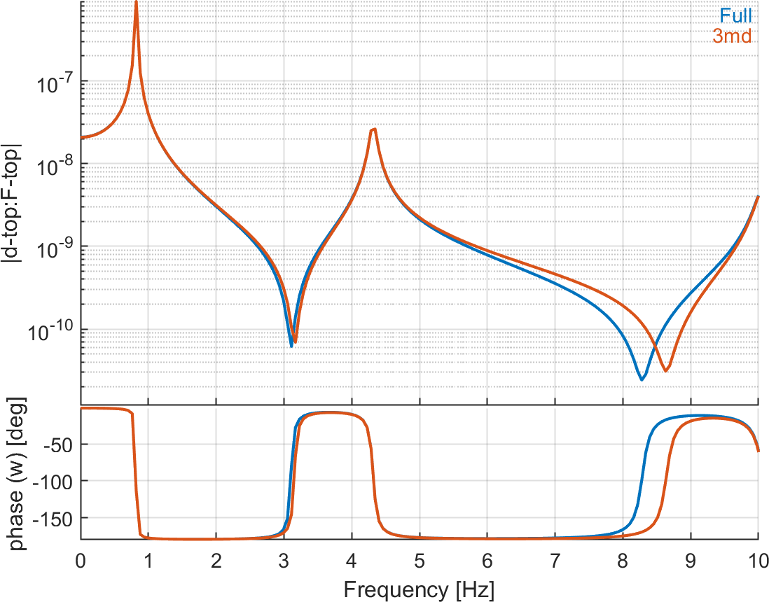
The transfer function computed with the full model is compared to the reduced model using only the first three modes of the beam in Figure 6.2. The agreement is very good at the resonances (poles) but there are some discrepancies around ω=0 (not clearly visible due to the logarithmic scale) and close to the anti-resonances (zeros). This is due to the contribution of the modes at higher frequencies which are not taken into account.
Frequency response functions are more efficiently computed using fe_simul in SDT. The general strategy to follow if one wants to use this function to compute the response of any given reduced model is to call fe_reduc. Several model reduction methods exist in the native function, but if one wants to implement another strategy, it is possible to call an external function. As using only mode shapes for model reduction is not accurate enough, this strategy is not implemented in fe_reduc.
In d_piezo('TutoPzTowerRed-s3')
, we show how to call an external function to build a reduced basis consisting only of the first N modes of a structure (here N=3). The results obtained are identical to the direct explicit approach (Figure 6.2).
%% Step 3 - Compute with fe_simul Full/3md

% Full model response
C0=fe_simul('dfrf -sens',stack_set(model,'info','Freq',w/(2*pi)));
% -sens option projects result on sensors only
C0.name='Full'; C0.X{2}={'d-top'}; C1.X{3}={'F-top'};

% With reduced basis 3 modes
model = stack_set(model,'info','EigOpt',[5 3 0]); % To keep 3 modes
% Build super-element with 3 modes
SE1=fe_reduc('call d_piezo@modal -matdes 2 1 3 4',model);

% Make model with a single super-element
SE0 = struct('Node',[],'Elt',[]);
mo1 = fesuper('SEAdd 1 -1 -unique -initcoef -newID se1',SE0,SE1) ;

% Define input/output
mo1=fe_case(mo1,'SensDOF','Output',21.01);
mo1=fe_case(mo1,'DofLoad','Input',21+.01,1);

% Compute response with fe_simul
C1=fe_simul('dfrf -sens',stack_set(mo1,'info','Freq',w/(2*pi)));
C1.name='3md+SE'; C1.X{2}={'d-top'};
It requires to build a function modal.m which is called by fe_reduc, the script of this function is given below:
function SE=modal()
%% just modal

% Transfers model to function
eval(iigui({'model','Case'},'MoveFromCaller'))
eval(iigui({'RunOpt'},'GetInCaller'))

% clean up model to remove info about matid/proid
SE=feutil('rmfield',model,'pl','il','unit','Stack');

% Compute modeshapes
def=fe_eig({model.K{1},model.K{2},Case.T, ...
   Case.mDOF},stack_get(model,'info','Eigopt','g'));

% reduce matrics based on N modes
SE.K = feutilb('tkt',def.def,model.K);
SE.DOF=[1:size(SE.K{1},1)]'+.99; % .99 DOFS
SE.Klab={'m' 'k' 'c' '4'};
SE.TR=def; SE.TR.adof=SE.DOF;

% assign to output
assignin('caller','T',SE)
assignin('caller','Case','');
The truncation error can be drastically reduced using static correction.
In d_piezo('TutoPzTowerRed-s4')
, a new reduced basis is therefore computed using fe_norm to orthogonalize the basis with respect to [K] and [M]. This is illustrated using low level calls.
%% Step 4 : Reduced basis 2 : 3 modes + static corr - explicit

Tstat=K\b;
T=fe_norm([def.def(:,1:3) Tstat],M,K); % Orthonormalize vectors

% Reduced matrices
Kr=T'*K*T; Mr=T'*M*T; br=T'*b;

% Ref solution
for i1=1:length(w)
     Ur2(:,i1)=(Kr*(1+0.02*1i)-w(i1)^2*Mr)\br;
end

out3=cta*(T*Ur2);

C2m=d_piezo('BuildC1',w'/(2*pi),out3.','d-top','F-top'); C2m.name='3md+Stat';
iicom(ci,'curveinit',{'curve',C0m.name,C0m;'curve',C2m.name,C2m});
iicom('submagpha'); d_piezo('setstyle',ci);
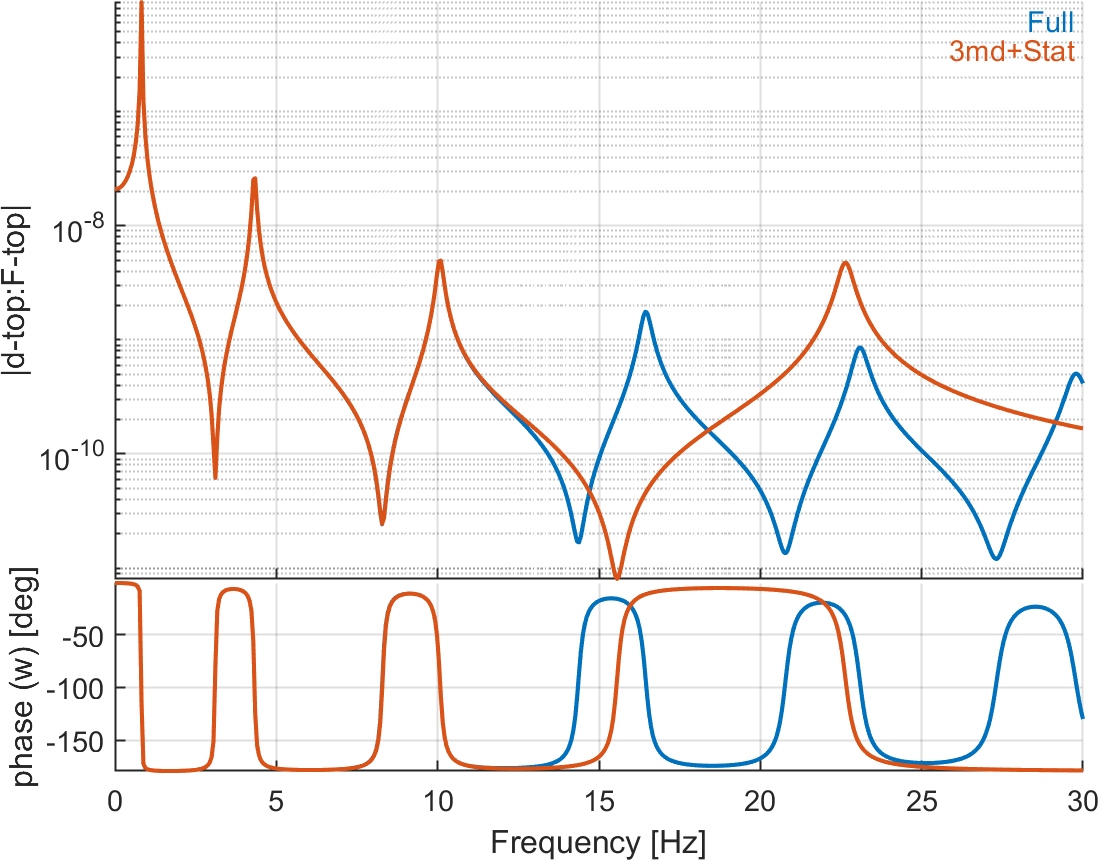
The transfer function computed using the static correction to the applied load is represented in Figure 6.3 in the extended frequency range from 0 to 30 Hz. The figure shows that the match is now excellent from 0 to 10 Hz. The static response and the anti-resonances (zeros) are predicted accurately. This is very important for active vibration control applications where the frequencies of the zero play a major role for predicting the performance of the active control scheme implemented.
Extending the frequency range for computations allows to show the behavior of the model at higher frequencies, and illustrates the fact that an additional non-physical mode is present when using normal modes
and static correction, whose contribution in the frequency band of interest is the same as the combination of all the contributions of the higher frequency modes for the full model.
Note that the first zero after the three modes in the frequency band of interest is not correct, even with the static correction.
The model reduction with N modes + static correction is natively implemented in the fe_reduc as illustrated in d_piezo('TutoPzTowerRed-s5')
%% Step 5 with fe_simul
model=d_piezo('meshtower');
model = stack_set(model,'info','EigOpt',[5 3 0]); % To keep 3 modes

% Reduce model with 3 modes and static correction
mo1=fe_reduc('free -matdes -SE 2 1 3 4 -bset',model);
% Compute response with fe_simul and represent
C2=fe_simul('dfrf -sens',stack_set(mo1,'info','Freq',w/(2*pi))); %
C2.name='3md+Stat-SE'; C2.X{2}={'d-top'};
ci=iiplot;iicom(ci,'curveinit',{'curve',C0.name,C0;'curve',C2.name,C2});
iicom('submagpha'); d_piezo('setstyle',ci);
It gives identical results as the direct explicit computation (Figure 6.3).
If the number of modes in the frequency band of interest becomes large, the technique becomes much more costly: the eigenvalue solver will need to compute more mode shapes, which increases strongly the computational time, and the number of equations to solve is also high. Usually, as the frequency increases, the modal density increases as well, so that the modal projection technique is not efficient anymore.