
 PDF Index
| SDT-visc
Contents
Functions
PDF Index |
Different major applications use families of structural models. Update problems, where a comparison with experimental results is used to update the mass and stiffness parameters of some elements or element groups that were not correctly modeled initially. Structural design problems, where component properties or shapes are optimized to achieve better performance. Non-linear problems where the properties of elements change as a function of operating conditions and/or frequency (viscoelastic behavior, geometrical non-linearity, etc.).
A family of models is defined (see [49] for more details) as a group of models of the general second order form (??) where the matrices composing the dynamic stiffness depend on a number of design parameters p
| (4.5) |
Moduli, beam section properties, plate thickness, frequency dependent damping, node locations, or component orientation for articulated systems are typical p parameters. The dependence on p parameters is often very non-linear. It is thus often desirable to use a model description in terms of other parameters α (which depend non-linearly on the p) to describe the evolution from the initial model as a linear combination (called zCoef in SDT)
| (4.6) |
with each [Zjα(s)] having constant mass, damping and stiffness properties.
Plates give a good example of p and α parameters. If p represents the plate thickness, one defines three α parameters: t for the membrane properties, t3 for the bending properties, and t2 for coupling effects.
p parameters linked to elastic properties (plate thickness, beam section properties, frequency dependent damping parameters, etc.) usually lead to low numbers of α parameters so that the α should be used. In other cases (p parameters representing node positions, configuration dependent properties, etc.) the approach is impractical and p should be used directly.
SDT handles parametric models where various areas of the model are associated with a scalar coefficient weighting the model matrices (stiffness, mass, damping, ...). The first step is to define a set of parameters, which is used to decompose the full model matrix in a linear combination.
The elements are grouped in non overlapping sets, indexed m, and using the fact that element stiffness depend linearly on the considered moduli, one can represent the dynamic stiffness matrix of the parameterized structure as a linear combination of constant matrices
| (4.7) |
Parameters are case stack entries defined by using fe_case par commands (which are identical to upcom Par commands for an upcom superelement).
A parameter entry defines a element selection and a type of varying matrix. Thus
 model=demosdt('demoubeam');
 model=fe_case(model,'par k 1 .1 10','Top','withnode {z>1}');
 fecom('proviewon');fecom('curtabCase','Top') % highlight the area
The weighting coefficients in (4.7) are defined formally using the
cf.Stack{'info','zCoef'} cell array viewed in the figure and detailed below.
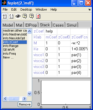
The columns of the cell array, which can be modified with the feplot interface, give
Given a model with defined parameters/matrices, model=fe_def('zcoef-default',model) defines default parameters.
zcoef=fe_def('zcoef',model) returns weighting coefficients for a range of values using the frequencies (see Freq) and design point stack entries
Frequencies are stored in the model using a call of the form model=stack_set(model,'info','Freq',w_hertz_colum). Design points (temperatures, optimization points, ...) are stored as rows of the 'info','Range' entry, see fevisco Range for generation.
When computing a response, fe_def zCoef starts by putting frequencies in a local variable w (which by convention is always in rd/s), and the current design point (row of 'info','Range' entry or row of its .val field if it exists) in a local variable par. zCoef2:end,4 is then evaluated to generate weighting coefficients zCoef giving the weighting needed to assemble the dynamic stiffness matrix (4.7). For example in a parametric analysis, where the coefficient par(1) stored in the first column of Range. One defines the ratio of current stiffness to nominal Kvcurrent=par(1)*Kv(nominal) as follows
% external to fexf
 zCoef={'Klab','mCoef','zCoef0','zCoefFcn';
        'M'    1       0        '-w.^2';
        'Ke'   0       1        1+i*fe_def('DefEta',[]);
        'Kv'   0       1        'par(1)'};
model=struct('K',{cell(1,3)});
model=stack_set(model,'info','zCoef',zCoef);
model=stack_set(model,'info','Range', ...
   struct('val',[1;2;3],'lab',{{'par'}}));

%Within fe2xf
w=[1:10]'*2*pi;  % frequencies in rad/s
Range=stack_get(model,'info','Range','getdata');
for jPar=1:size(Range.val,1)
 Range.jPar=jPar;zCoef=fe2xf('zcoef',model,w,Range);
 disp(zCoef)
  % some work gets done here ...
end
The viscoelastic tools handle parametric models where various areas of the model are associated with a scalar coefficient weighting the model matrices (stiffness, mass, damping, ...). The first step is to define a set of parameters, which is used to decompose the full model matrix in a linear combination. The elements are grouped in non overlapping sets, indexed m, and using the fact that element stiffness depend linearly on the considered moduli, one can represent the dynamic stiffness matrix of the parameterized structure as a linear combination of constant matrices
| (4.8) |
By convention, Ke represents the stiffness of all elements not in any other set. While the architecture is fully compatible there is no simplified mechanism to parameterize the mass.
The first step of a study is thus to define parameters. For all models this can be done using fe_case par commands (or upcom Par commands for an upcom superelement).
 model=demosdt('demoubeam');
 model=fe_case(model,'par','Top','withnode {z>1}');
 fecom('proviewon');fecom('curtabCase','Top') % highlight the area
If the parameters correspond to viscoelastic materials, one needs to declare which, of the initially elastic materials, are really viscoelastic. This is done using fevisco AddMat calls which associate particular MatId values with viscoelastic materials selected in the m_visco database.
 Up=d_visco('MeshPlate upreset');cf=feplot(Up);Up=cf.mdl;
 Up=stack_rm(Up,'mat');
 Up = fevisco('addmat 101',Up,'First area','ISD112 (1993)');
 Up = fevisco('addmat 103',Up,'Second area','ISD112 (1993)');
 cf.Stack{'info','Range'}=[20];
 cf.Stack{'info','Freq'}=logspace(1,3,30);
 %reset default zCoef Fcn and display
 fe2xf('zCoef-default',cf);fe2xf('zCoef',cf)
Viscoelastic materials are then considered as parameters by fevisco.
The full constant matrices M,Ke,Kvm can be assembled using fevisco MakeModel or with a NASTRAN DMAP fevisco Step12 (for implementations with other software such as ABAQUS, ANSYS or SAMCEF please contact us).
The normal mode of operation is to display your full model in a feplot figure. Reduced models can be generated with fe2xf direct commands, or with a NASTRAN DMAP step12, reduced matrices are stored in the model stack as an 'SE','MVR' entry.
xxx
The problems handled by fe2xf and computations at multiple frequencies and design points. Frequencies are either stored in the model using a call of the form model=stack_set(model,'info','Freq',w_hertz_colum) or given explicitly as an argument (the unit is then rad/s).
Design points (temperatures, optimization points, ...) are stored as rows of the 'info','Range' entry, see fevisco Range for generation.
When computing a response, fe2xf zCoef starts by putting frequencies in a local variable w (which by convention is always in rd/s), and the current design point (row of 'info','Range' entry or row of its .val field if it exists) in a local variable par. zCoef2:end,4 is then evaluated to generate weighting coefficients zCoef giving the weighting needed to assemble the dynamic stiffness matrix (4.7). For example in a parametric analysis, where the coefficient par(1) stored in the first column of Range. One defines the ratio of current stiffness to nominal Kvcurrent=par(1)*Kv(nominal) as follows
% external to fexf
 zCoef={'Klab','mCoef','zCoef0','zCoefFcn';
        'M'    1       0        '-w.^2';
        'Ke'   0       1        1+i*fe_def('DefEta',[]);
        'Kv'   0       1        'par(1)'};
model=struct('K',{cell(1,3)});
model=stack_set(model,'info','zCoef',zCoef);
model=stack_set(model,'info','Range', ...
   struct('val',[1;2;3],'lab',{{'par'}}));

%Within fe2xf
w=[1:10]'*2*pi;  % frequencies in rad/s
Range=stack_get(model,'info','Range','getdata');
for jPar=1:size(Range.val,1)
 Range.jPar=jPar;zCoef=fe2xf('zcoef',model,w,Range);
 disp(zCoef)
  % some work gets done here ...
end
To use a viscoelastic material, you can simply declare it using an AddMat command and use a '_visc' entry in the zCoefFcn column (the stack name for the material and the zCoef matrix name must match).
cf=d_visco('MeshPlateLoadMV feplot');
% define material with a unit conversion
mat=m_visco('convert INSI',m_visco('database Soundcoat-DYAD609'));
%                 MatId for original, name of parameter
cf.mdl = fevisco('addmat 101',cf.mdl,'Constrained 101',mat);
cf.Stack{'zCoef'}(4,4)={'_visc'};
% Third coefficient will use material with name
cf.Stack{'zCoef'}{4,1}
fe2xf('zcoef',cf,500:10:4000,struct('val',5,'lab',{{'T'}}));
At time of computation, the matrix coefficient in (4.7) is found as Gm(s,T,σ0)/Gm0 where the reference modulus is found in the cf.Stack{'Constraint 101'}.pl entry. The choice of E or G is based on the existence of a 'type','E' or 'type','G' entry in the mat.nomo field. For such materials one assumes Poisson's ratio to be real and the considered viscoelastic material to have its stiffness dominated by either shear or compression. Based on this assumption, one considers the frequency dependence of either the shear or Young's modulus. The error associated to neglecting the true variation of other moduli is assumed to be negligible (methodologies to treat cases where this is not true are not addressed here).
Inputs at DOFs are declared as fe_case entries.
If you have stored full basis vectors when building a reduced model (MVR.TR field), you may often be interested in redefining your inputs. To do so, you can use fe_case commands to define your loads, and MVR=fe_sens('br&lab',MVR,model), to redefine the reduced inputs accordingly.
MV=d_visco('MeshPlate');
MV=fe_case(MV,'SensDof','BasicAtDof',[1;246]+.03);
% Surface velocity
'xxx'
% NEED TO BE REVISED WITH STRESS CUT 4 strain sensors along a line
%pos=linspace(.5,1,4)';pos(:,2)=.75; pos(:,3)=.006;
%data=struct('Node',pos,'dir',ones(size(pos,1),1)*[1 0 0]);
%MV=fe_case(MV,'SensStrain','ShearInLayer',data)
Sens=fe_case(MV,'sens')
If you have stored full basis vectors when building a reduced model (MVR.TR field), you may often be interested in redefining your sensors. To do so, you can use the fe_case commands to set your sensors, and fe_sens('cr&lab',cf) to redefine the reduced sensors accordingly (this calls Sens=fe_case('sens',model) to generate the data structure combining the observation equations of all your sensors).
 [MV,cf]=d_visco('MeshPlateLoadMVR');cf.Stack{'MVR'}
 % redefine sensors
 i1=feutil('findnode x==0 & z==0 epsl1e-3',MV);
 MV=fe_case(MV,'SensDof','Sensors',i1+.03);
 % reset reduced sensor representation
 fe_sens('cr&lab',cf);cf.Stack{'MVR'}
A viscoelastic model (see section 4.5.6 for the typical generation procedure), stores the information needed to compute (4.7) in a data structure stored as a SE,MVR stack entry. The format corresponds to a generic type 1 superelement (handled by fe_super) but the following fields are specifically of interest.
| .Opt | Options characterizing the model matrices. In particular the second row describes the type of each matrix in model.K (1 for stiffness, 2 for mass, ... ) |
| .K | a cell array of matrices giving the constant matrices in (4.7). One normally uses M,Ke,Kvm, .... These matrices should be real and only the combination coefficients should be complex. |
| .Klab | a cell array giving a labels for matrices in the .K field. |
| .DOF | DOF definition vector associated with matrices in .K |
| .Stack | standard model stack where one defines viscoelastic materials (see fevisco AddMat and m_visco database), frequencies, zcoef, reduced model, range (see fevisco Range) ... as well as the case that contains descriptions for loads, sensors, parameters, ... |
Additional fields used in some solutions are
| .br | input shape matrix for reduced model, generated by fe_sens('br&lab',MVR). |
| .cr | input shape matrix for reduced model, generated by fe_sens('cr&lab',MVR). |
| .kd | optional static preconditioner (nominally equal to ofact(k0)) use to compute static response based on a known residue. Deprecated and replaced by fe2xf Build calls. |
For a given reduced (or full) model you may want to post-process the computed frequency responses before saving them. This is in particular important to analyze responses on large sensor sets (panel velocities, stresses, ...) which would require a lot of storage space if saved at all frequencies.
The list MifDes xxx


