Sample setup for parametric studies

SDT-visc Contents Functions

PDF Index

4.5 Sample setup for parametric studies

This section provides tutorial studies based on SDT-visc only.

4.5.1 Performance in modulus/loss plane

This tutorial uses the cantilever constrained plate shown in the figure below.

Figure 4.1: Constrained layer model validity.

d_visco('TutoEhPerf-s1') meshes a cantilever constrained plate.

step 2 builds a reduced model. One starts by defining a viscoelastic material, and then uses an fe2xf Build call to build the reduced model by learning a soft and a stiff modulus point.

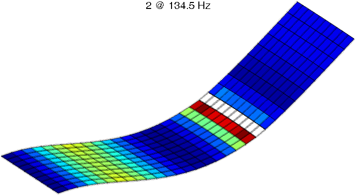
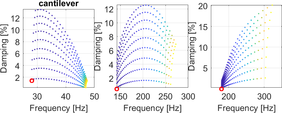
step 3 generates the standard frequency/damping curves for the first 3 modes.

With EhPerf one obtains the damping level as function of modulus and loss factor map. In the present case one sees that the best performance is obtained for a modulus around 2 MPa.

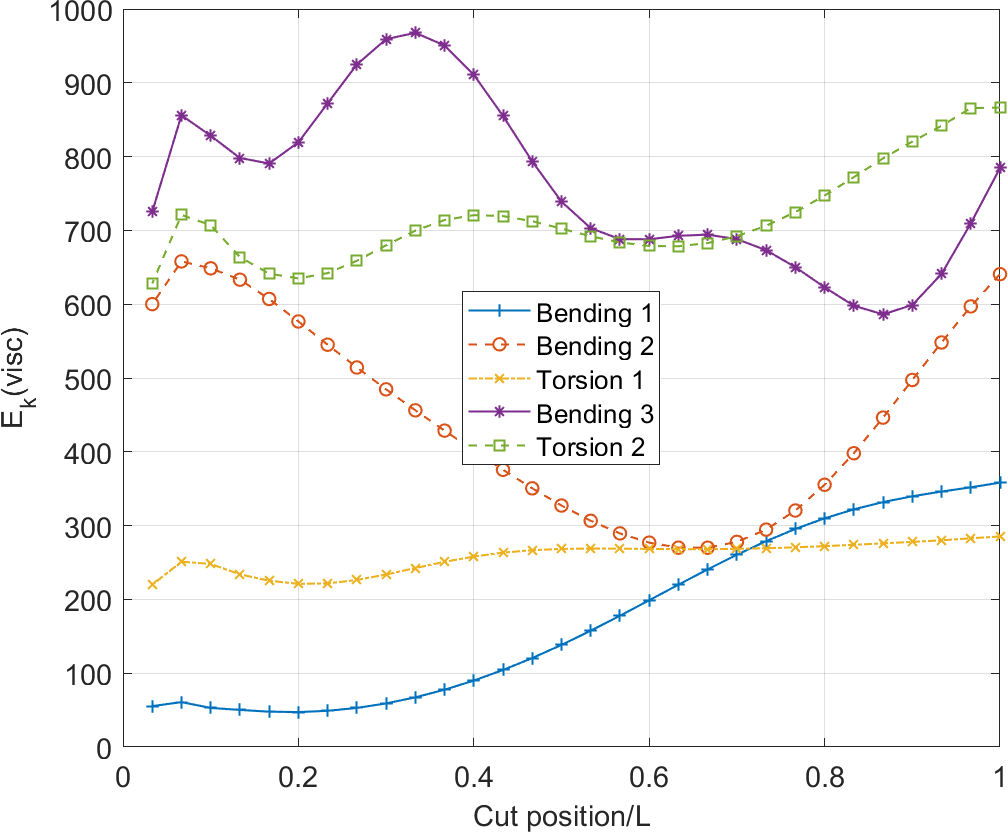
The data used for the E,η performance map is a grid which for each mode can be shown in the frequency damping plane as illustrated below

It may also be interesting to split those maps by mode as shown here.

Older demos are basic_sandwich which generates curves for the validation of shell/volume/shell model used to represent constrained layer treatments as first discussed in section ??.

4.5.2 Illustration of pole range computations

d_visco('TutoPoleRange-s1') uses a beam with viscoelastic rotational spring example.

4.5.3 Model parameterization

fevisco handles parametric models with variable stiffness expressed as linear combinations of constant matrices (??). The initial step of all parametric studies is to define the parameter sets.

For example, a selection based on ProId.

 model=fe_case(model,'par','FrontStruts','-k ProId 168';
                     'par','BackStruts' ,'-k ProId 304'};

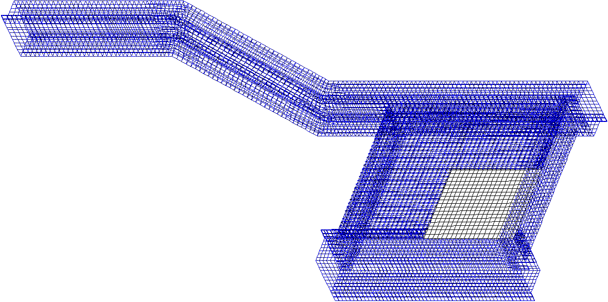
The PREDIT_mat model XXX

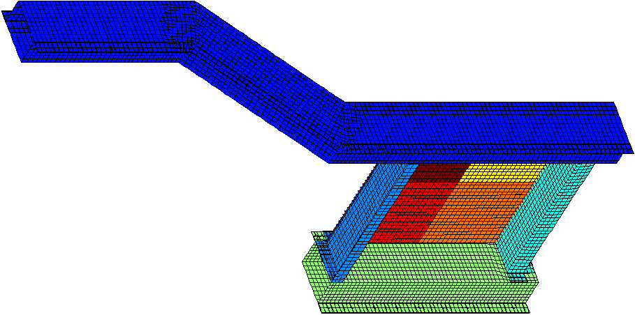
Figure 4.2: The PREDIT_mat model

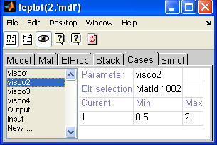
For example, in the PREDIT_mat model, one can define each of the 4 squares of viscoelastic materials on the pane as a parameter using ProId

 cf=feplot(model); MV=cf.mdl; %XXX

One can then visualize each parameter using feplot model properties windows, within the Case tab

4.5.4 Sample parametric study in SDT (full solver, Upcom superelement)

Typically, one starts predictions with the a first order approximation to generate a reduced model MVR which is then used to approximate the frequency response functions Rred

 Up=fevisco('testplate upreset');
 %Up=fevisco('testplate up');
 Up=stack_rm(Up,'mat');
 Up = fevisco('addmat 101',Up,'Area1','ISD112 (1993)');
 Up = fevisco('addmat 103',Up,'Area2','ISD112 (1993)');
 MV=fevisco('makemodel matid 101 103',Up);  
 cf=feplot(MV);
 cf.Stack{'info','Range'}=[10;30];
 cf.Stack{'info','Freq'}=[30:.5:500]';   % Target frequencies Hz
 cf.Stack{'info','EigOpt'}=[6 40 -(2*pi*30)^2 11];
 fe2xf('directfirst zCoef0',cf);  
 ci=iiplot(cf.Stack{'curve','RESP'});
 iicom('challDesign point')

 % This is a call to the new strategy for pole tracking as function of temp
 RO=struct('IndMode',7:20,'Temp',20:10:100,'Freq',logspace(1,4,20)');
 Po=fevisco('poletemp',cf,{'Area1';'Area2'},RO);
 fe2xf('plotpolesearch',Po)

This is a sample direct computation of the viscoelastic response at 3 frequencies.

fevisco('testplate matrix');cf=feplot;MV=cf.mdl;
cf.Stack{'info','Freq'}=[5:5:40]';
 [Rfull,def]=fe2xf('directfull',MV);  
 cf.def=def; % NEED REVISE : iiplot(Rfull);

Given the reduced model MVR you can then track poles through your parametric range using

 MVR.Range=[0:10:50]';
 Hist=fe2xf('frfpolesearch',MVR);
 fe2xf('plotpolesearch',Hist) % Generate standard plot of result

4.5.5 Parametric model generated within NASTRAN (fo_by_set DMAP)

The following gives a simple example of a beam separated in two parts. The step12 calls run NASTRAN with the fo_by_set DMAP where an eigenvalue computation is used to generate a modal basis that is then enriched (so called step 1) before generating a parametric reduced model (step 2).

The steps of the procedure are the following

load the initial model into MATLAB using a nasread command.
Generate through naswrite commands, or manual editing, a RootName_bulk.bdf file that contains bulk data information, EIGRL and and possibly PARAM cards.
NOTE elements that will be parameterized should have the loss factor of their material set to zero.
Define element groups associated with parameters (see section ??).
These can be easily checked using feplot (open the Edit:Model properties menu and go to the Case tab). cf.sel=selection{1,2} commands. Once the job is written, elements sets will be written in a parameter_sets.bdf file (using nas2up WriteSetC commands).
Sensors using SensDof case entries, see section ??.
Generate the RootName_step12.dat file and run the job using
```
  cf=feplot; % the model should be displayed in feplot
  cf.mdl=nas2up('JobOpt',cf.mdl); % Init NasJobOpt entry to its default
  fevisco('writeStep12 -run','RootName',cf)
  fecom(cf,'Save','FileName'); % save your model for reload
```
where the write command edits the nominal job files found in sdtdef('FEMLink.DmapDir')).
If you need to edit the bulk file, for job specific aspects of the Case Control Section (definition of MPC and SPC for example), omit the -run, do your manual edits, then run the job (for example nas2up('joball memory=8GB','RootName_step12.dat').
You can also pre-specify a series of EditBulk entries so that your job can run automatically. For example
```
edits={'insert',   'SOL 103'        ,'', 'GEOMCHECK NONE';
       'replace', 'SPC        = 10','', 'SPC        = 1'};
model=stack_set(model,'info','EditBulk',edits);
```
Once the NASTRAN job done, you should have locally the files RootName_mkekvr.op4 (reduced matrices), RootName_USETT.op2 degree of freedom set and info needed to build Case.T, RootName_TR.op4 basis vectors defined on DOFs that are needed (sensor and input DOFs).
You are now ready to build the reduced parameterized model using
```
 cf=feplot;fecom(cf,'Load','FileName');
 MVR=fevisco('BuildStep12','RootName',model)
```
If the files are not automatically copied from the NASTRAN server machine, the BuildStep12 -cpfrom makes sure the result file are copied back.

Here is a complete example of this procedure

 cd(sdtdef('tempdir')); if ~isunix; return;end % Don't test on windows
 wd=sdtdef('FEMLink.DmapDir-safe',fullfile(fileparts(which('nasread')),'dmap'));
 copyfile(fullfile(wd,'fo*.dmp'),'.')
 copyfile(fullfile(wd,'sdt*.dmp'),'.')
 !rm ubeam_step12.MASTER ubeam_step12.DBALL ubeam_*.[0-9]

 model=demosdt('demoubeam');cf=feplot;
 model=fe_case(model,'dofload','Input', ...
  struct('DOF',[349.01;360.01;241.01;365.03],'def',[1;-1;1;1],'ID',100));
 model=fe_case(model,'par','Top','withnode {z>1}');
 model=fe_case(model,'sensdof','Sensors',[360.01]);
 cf.Stack{'info','EigOpt'}=[5 20 1e3 11];
 model=nas2up('JobOpt',model); % Init NasJobOpt entry to its default
 cf.Stack{'info','Freq'}=[20:2:150];
 fevisco('writeStep12 -write -run','ubeam',model);
 fecom('save','ubeam_param.mat'); % save before MVR is built
 % you may sometimes need to quit Matlab here if NASTRAN is long
 cf=feplot('Load','ubeam_param.mat'); % reload if you quit matlab
 fevisco('BuildStep12','ubeam',cf) 
 fecom('save','ubeam_param.mat'); % save after MVR is built

When dealing with a model that would have been treated through a SOL108 (full order direct frequency response), the parametric model returns a B matrix. This is actually related to the K_e and K_vi matrices by

(4.9)

where η_glob is defined in NASTRAN using PARAM,G and the loss factors for the viscoelastic parts using the GE values of the respective components.

For viscoelastic analysis NASTRAN requests a complex curve T(ω) given as two tables. NASTRAN applies the PARAM,G to all elements (the matrix called K_dd¹ in NASTRAN lingo is equal to K_e+∑_i K_vi) as a result the variable viscoelastic stiffness which are here proportional to G(ω)/G_i,nom = 1+iη_glob + T(ω) η_i,nom hence, given the complex modulus, the table is given by

(4.10)

Generation of variable coefficients to be used in the toolbox from NASTRAN input is obtained with MVR.zCoefFcn=fevisco('nastranzCoefv1',model).

4.5.6 Parametric model from NASTRAN element matrices

An alternative to the step12 procedure Viscoelastic computations are performed on an upcom model typically imported from NASTRAN after a SOL103 (real eigenvalue) run with PARAM,POST,-4 to export the element matrices. Thus for a NASTRAN run UpModel.dat which generated UpModel.op2 and where the upcom superelement is saved in UpModel.mat a typical script begins with Up=nasread('UpModel.dat','BuildOrLoad').

In some cases, one may want to use reduced basis vectors that are generated by an external code (typically NASTRAN). The problem is then to generate the reduced model MVR without asking fevisco to generate the appropriate basis. You can simply call the DirectReduced command

 Up=fevisco('testplate upreset');
 Up=stack_rm(Up,'mat');
 Up = fevisco('addmat 101',Up,'First area','ISD112 (1993)');
 Up = fevisco('addmat 103',Up,'Second area','ISD112 (1993)');

 def=fe_eig(Up,[6 10 1e3]);
 MVR = fevisco('makemodel matid 101 103',Up,def); 
 MVR=stack_set(MVR,'info','Freq',[20:.5:90]'); 
 RESP=fe2xf('directreduced',MVR);  % Result in XF(1)