Design of an accelerometer and computation of its sensitivity

SDT-piezo Contents Functions

8.1 Design of an accelerometer and computation of its sensitivity

This application example deals with the determination of the sensitivity of a piezoelectric sensor to base excitation.

8.1.1 Working principle of an accelerometer

By far the most common sensor for measuring vibrations is the accelerometer. The basic working principle of such a device is presented in Figure 8.1(a). It consists of a moving mass on a spring and dashpot, attached to a moving solid. The acceleration of the moving solid results in a differential movement x between the mass M and the solid. The governing equation is given by,

(1)

In the frequency domain x/x₀ is given by,

(2)

with ω_n = √k/M and ξ=b/2√kM and for frequencies ω << ω_n, one has,

(3)

showing that at low frequencies compared to the natural frequency of the mass-spring system, x is proportional to the acceleration x₀. Note that since the proportionality factor is −1/ω_n², the sensitivity of the sensor is increased as ω_n² is decreased. At the same time, the frequency band in which the accelerometer response is proportional to x₀ is reduced.

(a) (b)

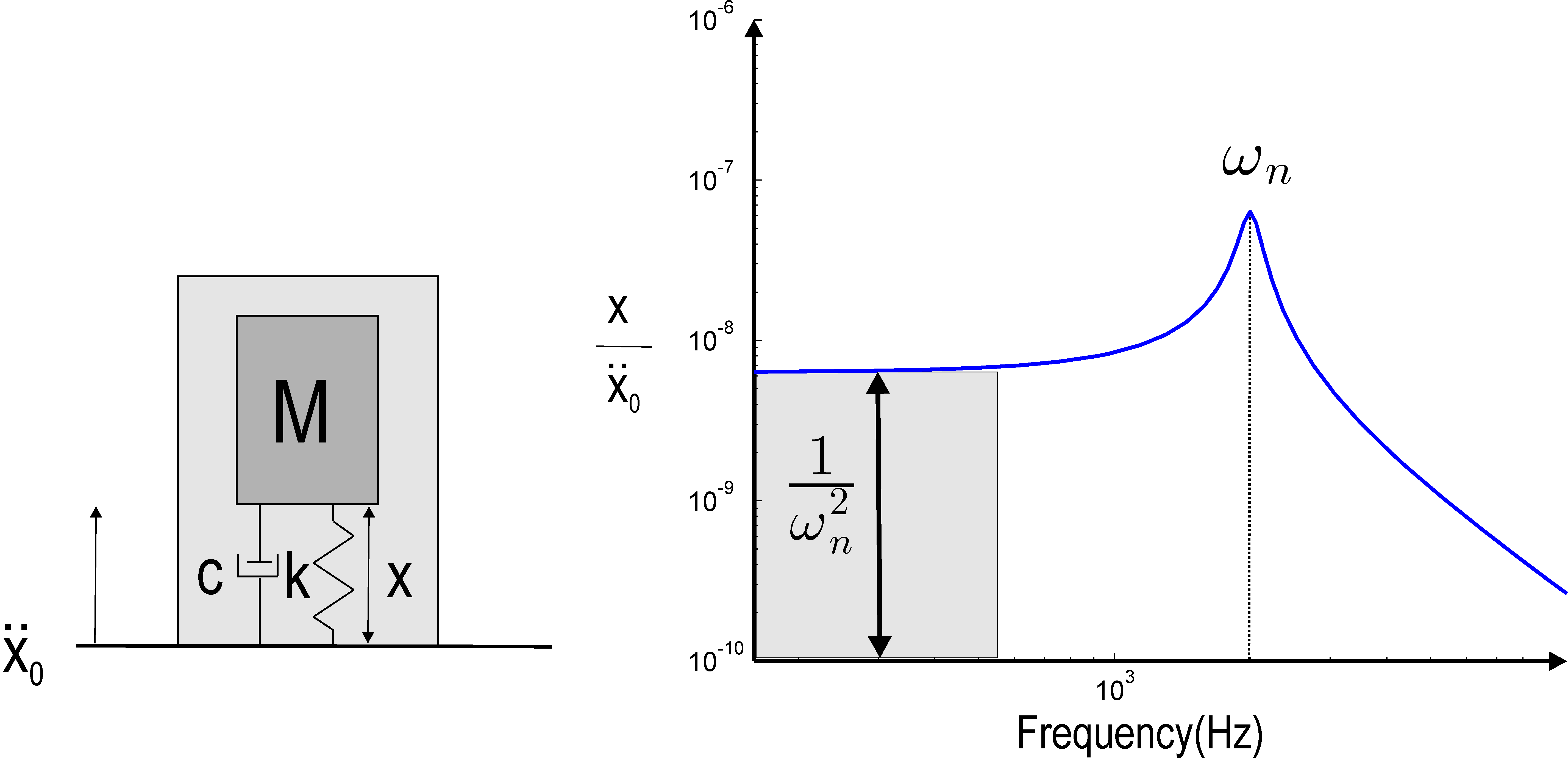
Figure 8.1: Working principle of an accelerometer

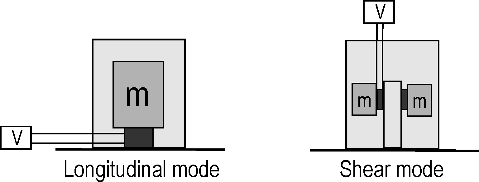
The relative displacement x can be measured in different ways among which the use of piezoelectric material, either in longitudinal or shear mode (Figure 8.2). In such configurations, the strain applied to the piezoelectric material is proportional to the relative displacement between the mass and the base. If no amplifier is used, the voltage generated between the electrodes of the piezoelectric material is directly proportional to the strain, and therefore to the relative displacement. For frequencies well below the natural frequency of the accelerometer, the voltage produced is therefore proportional to the absolute acceleration of the base.

Figure 8.2: Different sensing principles for standard piezoelectric accelerometers

8.1.2 Determining the sensitivity of an accelerometer to base excitation

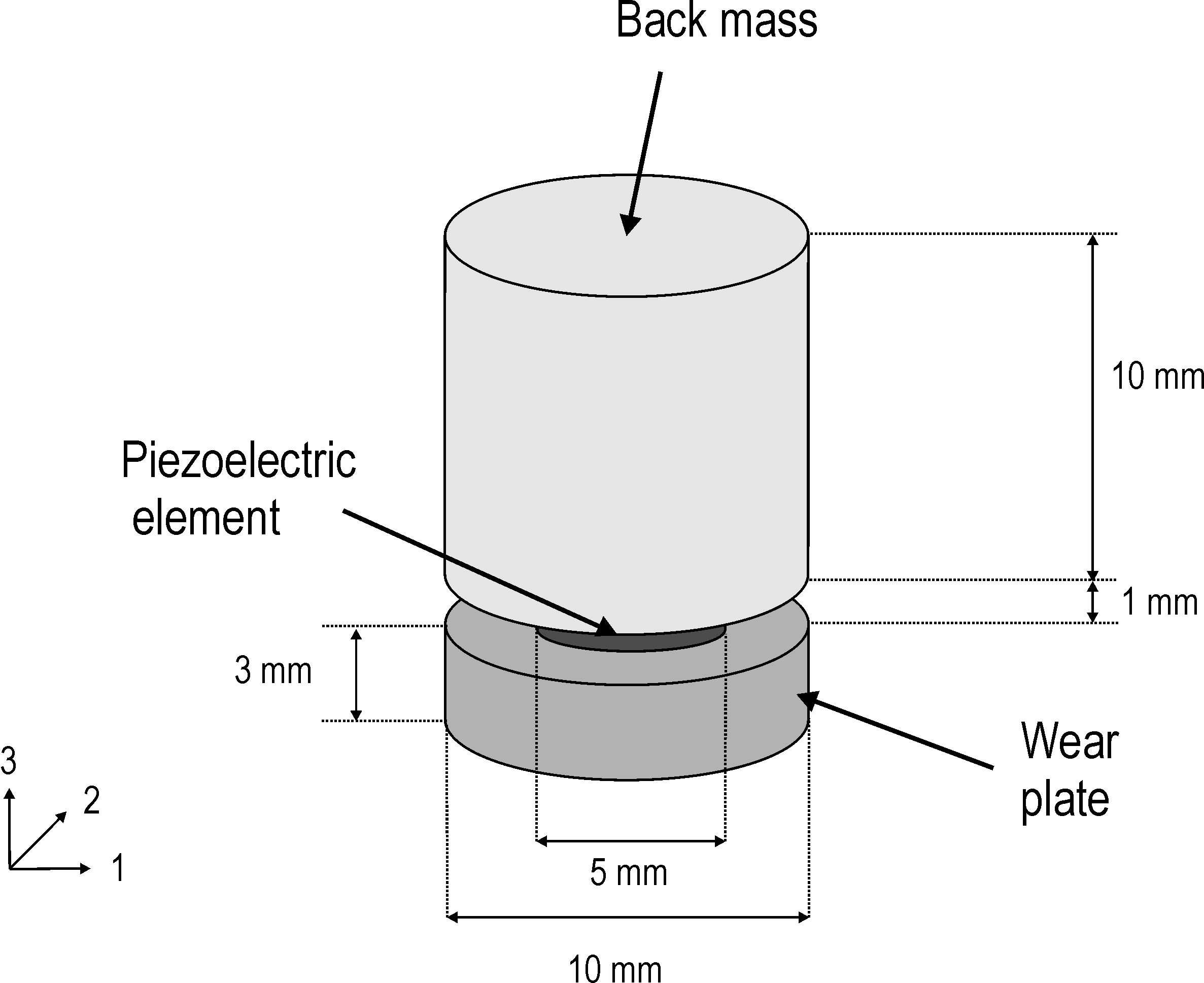
A basic design of a piezoelectric accelerometer working in the longitudinal mode is shown in Figure 8.3. In this example, the casing of the accelerometer is not taken into account, so that the device consists in a 3mm thick rigid wear plate (10mm diameter), a 1mm thick piezoelectric element (5mm diameter), and a 10mm thick (10mm diameter) steel proof mass. The mechanical properties of the three elements are given in Table 8.1. The piezoelectric properties of the sensing element are given in Table 8.2 and correspond to SONOX_P502_iso property in m_piezo Database. The sensing element is poled through the thickness and the two electrodes are on the top and bottom surfaces.

Figure 8.3: Basic design of a piezoelectric accelerometer working in the longitudinal mode

Part Material E (GPa) ρ (kg/m³) ν

Wear plate Al₂O₃ 400 3965 0.22

Sensing element Piezo 54 7740 0.44

Proof mass Steel 210 7800 0.3

Table 8.1: Mechanical properties of the wear plate, sensing element and proof mass

Property Value

d₃₁=d₃₂ -185 10⁻¹² pC/N (or m/V)

d₃₃ 440 10⁻¹² pC/N (or m/V)

d₁₅=d₂₄ 560 10⁻¹² pC/N (or m/V)

є₃₃^T=є₂₂^T=є₁₁^T 1850 є₀

є₀ 8.854 10⁻¹² Fm⁻¹

Table 8.2: Piezoelectric properties of the sensing element

The sensitivity curve of the accelerometer, expressed in V/m/s² is used to assess the response of the sensor to a base acceleration in the sensing direction (here vertical). In order to compute this sensitivity curve, one needs therefore to apply a uniform vertical base acceleration to the sensor and to compute the response of the sensing element as a function of the frequency.
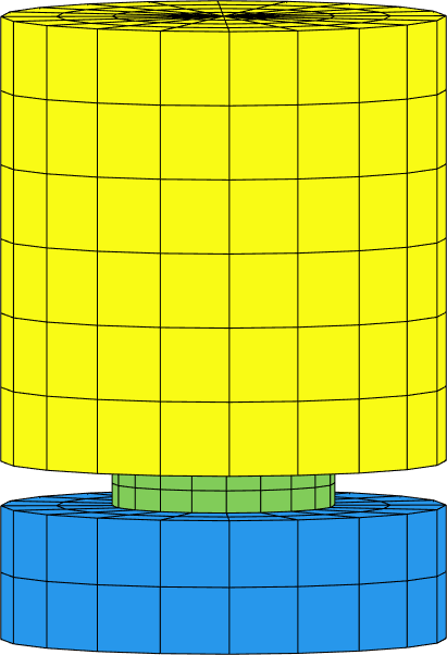
The mesh is built and visualized in d_piezo('TutoPzAccel-s1') . It is shown in Figure 8.4

Figure 8.4: Mesh of the piezoelectric accelerometer. The different colors represent the different groups

The call includes the meshing of the accelerometer, the definition of material properties, as well as the definition of electrodes. In addition, the bottom electrode is grounded, and both a voltage and a charge sensor are defined for the top electrode.
In d_piezo('TutoPzAccel-s2') , a displacement sensor at the center of the base is defined in order to compute the sensitivity.

%% Step 2 - Define sensors and actuators
% -MatID 2 requests a charge resultant sensor
% -vout requests a voltage sensor
model=p_piezo('ElectrodeMPC Top sensor -matid 2 -vout',model,'z==0.004');
% -ground generates a v=0 FixDof case entry
model=p_piezo('ElectrodeMPC Bottom sensor -ground',model,'z==0.003');
% Add a displacement sensor for the basis
model=fe_case(model,'SensDof','Base-displ',1.03);

The sensitivity for the sensor used in a voltage mode is then computed using an imposed displacement on the basis. The measured displacement is transformed to acceleration in the frequency domain.

It is represented in Figure 8.5 and is computed with the following script:
(d_piezo('TutoAccel-s3') )

%% Step 3 - Response with imposed displacement
% Remove the charge sensor (not needed)
model=fe_case(model,'remove','Q-Top sensor');

% Link dofs of base and impose unit vertical displacement
n1=feutil('getnode z==0',model);
rb=feutilb('geomrb',n1,[0 0 0],fe_c(feutil('getdof',model),n1(:,1),'dof'));
rb=fe_def('subdef',rb,3); % Keep vertical displacement
model=fe_case(model,'DofSet','Base',rb);

% Other parameters
f=linspace(1e3,2e5,200)';
model=stack_set(model,'info','Freq',f); % freq. for computation

 % Reduced ss-model
[sys,TR1]=fe2ss('free 5 10 0 -dterm',model,5e-3); %

C1=qbode(sys,f(:)*2*pi,'struct-lab');C1.name='SS-voltage';
C1.X{2}={'Sensor output(V)';'Base Acc(m/s^2)';'Sensitivity (V/m/s^2)'}; %outputs

% C1 compute accel and sensitivity
 C1.Y(:,2)=C1.Y(:,2).*(-(C1.X{1}*2*pi).^2); % Base acc
 C1.Y(:,3)=C1.Y(:,1)./C1.Y(:,2);% Sensitivity
 
 ci=iiplot; iicom(ci,'curveinit',{'curve',C1.name,C1});  iicom('ch3');
 d_piezo('setstyle',ci)

Figure 8.5: Sensitivity of the accelerometer in the voltage mode, uniform acceleration imposed at the base

The sensor can also be used in the charge mode. The following scripts compares the sensitivity of the sensor used in the voltage and charge modes. The sensitivities are normalized to the static sensitivity in order to be compared on the same graph, as the orders of magnitude are very different (Figure 8.6). The charge sensor corresponds to a short-circuit condition which results in a lower resonant frequency than the sensor used in a voltage mode where the electric field is present in section 6.3.4 for a plate. Here the difference of eigenfrequency is however higher (about 10%) due to the fact that there is more strain energy in the piezoelectric element, and that it is used in the d₃₃ mode which has a higher electromechanical coupling factor than the d₃₁ mode.
(d_piezo('TutoPzAccel-s4') )

 %% Step 4 - Compare charge and voltage mode for sensing
 
model=d_piezo('MeshBaseAccel');
model=fe_case(model,'remove','V-Top sensor');

% Short-circuit electrodes of accelerometer
model=fe_case(model,'FixDof','V=0 on Top Sensor', ...
    p_piezo('electrodedof Top sensor',model));

% Other parameters
  model=stack_set(model,'info','Freq',f);

% Link dofs of base and impose unit vertical displacement
n1=feutil('getnode z==0',model);
rb=feutilb('geomrb',n1,[0 0 0],fe_c(feutil('getdof',model),n1(:,1),'dof'));
rb=fe_def('subdef',rb,3); % Keep vertical displacement
model=fe_case(model,'DofSet','Base',rb);

% Reduced model
[sys2,TR1]=fe2ss('free 5 10 0 -dterm',model,5e-3); %
C2=qbode(sys2,f(:)*2*pi,'struct');C2.name='SS-charge';

C2.X{2}={'Sensor output(V)';'Base Acc(m/s^2)';'Sensitivity (normalized)'}; %outputs
C1.X{2}={'Sensor output(q)';'Base Acc(m/s^2)';'Sensitivity (normalized)'};

% C2 compute accel and sensitivity
 C2.Y(:,2)=C2.Y(:,2).*(-(C2.X{1}*2*pi).^2); % Base acc
 C2.Y(:,3)=C2.Y(:,1)./C2.Y(:,2);% Sensitivity

 % Normalize sensitivity to first freq
 C1.Y(:,3)=C1.Y(:,3)/abs(C1.Y(1,3));
 C2.Y(:,3)=C2.Y(:,3)/abs(C2.Y(1,3))

 ci=iiplot; iicom(ci,'curveinit',{'curve',C1.name,C1;'curve',C2.name,C2}); ...
 iicom('ch3');  d_piezo('setstyle',ci)

Figure 8.6: Comparison of the normalized sensitivities of the sensor used in the charge and voltage mode

8.1.3 Computing the sensitivity curve using a piezoelectric shaker

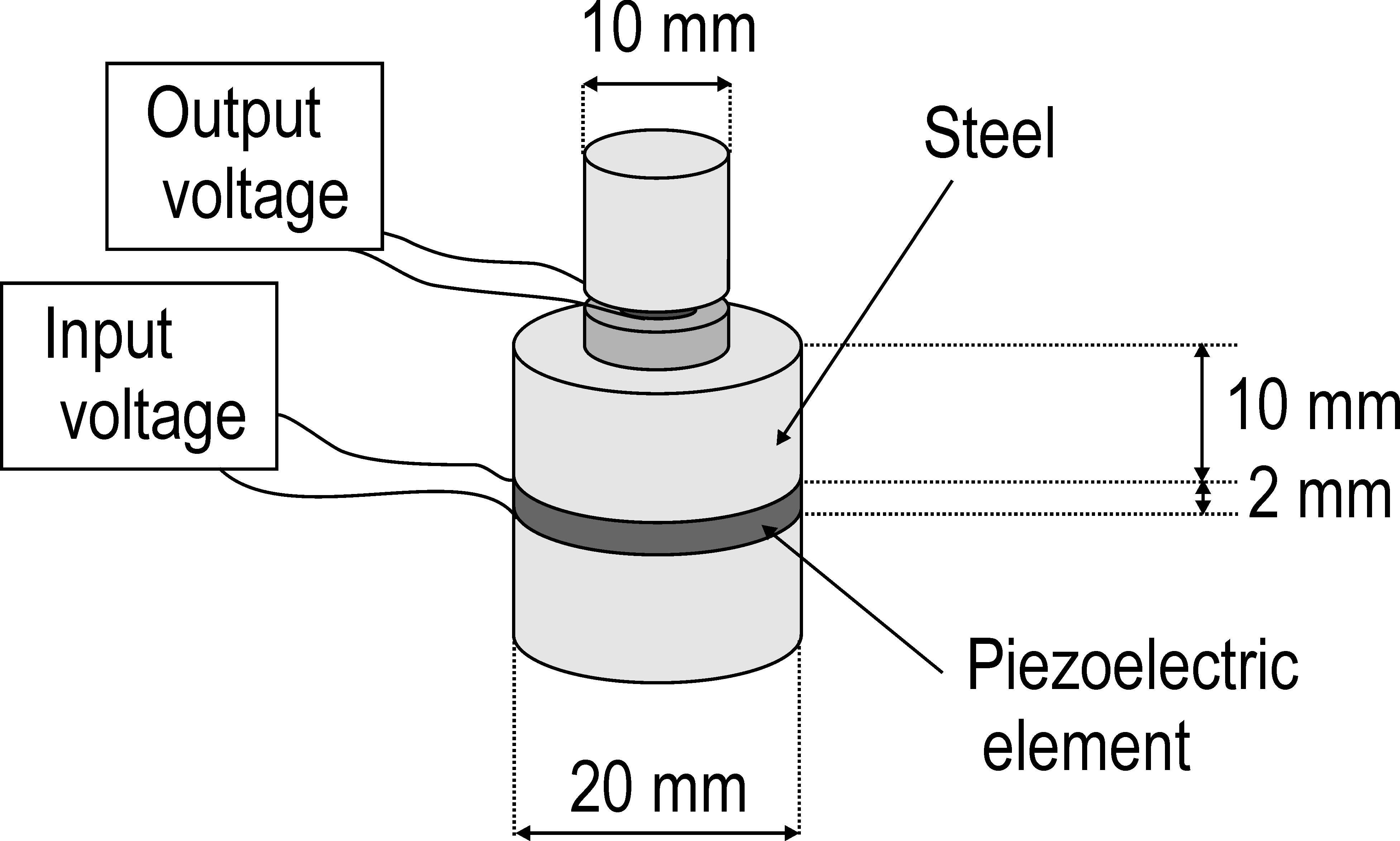
Experimentally, the sensitivity curve can be measured by attaching the accelerometer to a shaker in order to excite the base. Usually, this is done with an electromagnetic shaker, but we illustrate in the following example the use of a piezoelectric shaker for sensor calibration. The piezoelectric shaker consists of two steel cylindrical parts with a piezoelectric disc inserted in between. The base of the shaker is fixed and the piezoelectric element is used as an actuator: imposing a voltage difference between the electrodes results in the motion of the top surface of the shaker to which the accelerometer is attached (Figure 8.7).

Figure 8.7: Piezoelectric accelerometer attached to a piezoelectric shaker for sensor calibration

The piezoelectric properties for the actuating element in the piezoelectric shaker are identical to the ones of the sensing element given in Table 4.3 and it is poled through the thickness.
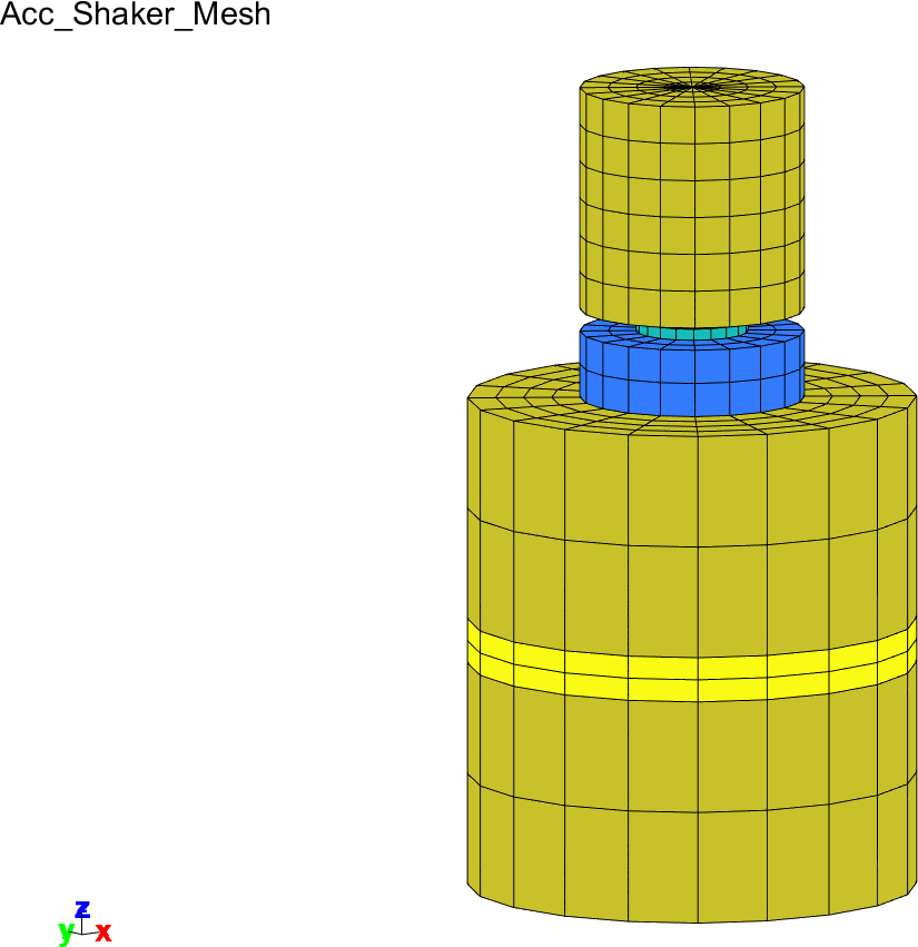
In d_piezo('TutoPzAccShaker-s1') , the mesh is produced and visualized (Figure 8.8).

Then in d_piezo('TutoPzAccShaker-s2') , a voltage actuator is defined for the piezoelectric disk in the piezoelectric shaker by setting the bottom electrode potential to zero, and defining the top electrode potential as an input, and an acceleration sensor is defined at the base of the accelerometer.

Figure 8.8: Mesh of the piezoelectric accelerometer attached to a piezoelectric shaker

d_piezo('TutoPzAccShaker-s3') is used to compute the response on the sensors (acceleration at the base of the accelerometer, and voltage on the piezo disk in the accelerometer) and to deduce the sensitivity of the accelerometer by dividing the sensor output by the base acceleration.

%% Step 3 - Compute response, voltage input on shaker
f=linspace(1e3,2e5,200)';
model=stack_set(model,'info','Freq',f);

% Reduced ss-model
model=fe_case(model,'pcond','Piezo','d_piezo(''Pcond'')');
[sys,TR1]=fe2ss('free 5 45 0 -dterm ',model,1e-3); %

C1=qbode(sys,f(:)*2*pi,'struct-lab');C1.name='SS-voltage';
C1.X{2}={'Sensor output(V)';'Base Acc(m/s^2)';'Sensitivity (V/m/s^2)'}; %outputs

% Compute sensitivity
C1.Y(:,3)=C1.Y(:,1)./C1.Y(:,2);% Sensitivity
 
ci=iiplot; iicom(ci,'curveinit',{'curve',C1.name,C1});  iicom('ch3');
d_piezo('setstyle',ci)

The sensitivity curve obtained is shown in Figure 8.9. It is comparable to the one computed with imposed displacement around the natural frequency of the accelerometer, but at low frequencies, the flat part is not correctly represented and a few spurious peaks appear at high frequencies. These differences are due to the fact that the piezoelectric shaker does not impose a uniform acceleration of the base of the sensor, and has several resonance frequencies in the band of interest. There are also lateral (contraction) effects due to the piezoelectric element in the shaker which induce a response of the accelerometer and modify the sensitivity curve.

Figure 8.9: Sensitivity curve obtained with a piezoelectric shaker


Part	Material	E (GPa)	ρ (kg/m³)	ν

Wear plate	Al₂O₃	400	3965	0.22
Sensing element	Piezo	54	7740	0.44
Proof mass	Steel	210	7800	0.3

Property	Value
d₃₁=d₃₂	-185 10⁻¹² pC/N (or m/V)
d₃₃	440 10⁻¹² pC/N (or m/V)
d₁₅=d₂₄	560 10⁻¹² pC/N (or m/V)
є₃₃^T=є₂₂^T=є₁₁^T	1850 є₀
є₀	8.854 10⁻¹² Fm⁻¹