
 PDF Index
| SDT-piezo
Contents
Functions
PDF Index |
In this very simple example, the electric field and the strains are all constant, so that the electric potential and the displacement field are linear. The example is treated analytically in section section 2.4. It is therefore possible to obtain an exact solution using a single volumic 8-node finite element (with linear shape functions, the nodal unknowns being the displacements in x,y and z and the electric potential φ). Consider a piezoelectric patch whose dimensions and material properties are given in Table 3.1. The material properties correspond to the material SONOX_P502_iso in m_piezo.
Property Value b 10 mm w 10 mm h 2 mm E 54 GPa ν 0.41 d31=d32 -185 10−12 pC/N (or m/V) d33 440 10−12 pC/N (or m/V) d15=d24 560 10−12 pC/N (or m/V) є33T=є22T=є11T 1850 є0 є0 8.854 10−12 Fm−1
Table 3.1: Geometrical and material properties of the piezoelectric patch
We first produce the mesh, associate the material properties and define the electrodes with
 d_piezo('TutoPzPatchExt-s1')
. The default material is SONOX_P502_iso. The number of elements in the x, y and z directions are given by nx,ny and nz.
d_piezo('TutoPzPatchExt-s1')
. The default material is SONOX_P502_iso. The number of elements in the x, y and z directions are given by nx,ny and nz.
The information about the nodes associated to each electrode can be obtained through the following call (Figure 3.4):
p_piezo('TabInfo',model)
In d_piezo('TutoPzPatchExt-s2')
, the material is changed for example to PIC_255 with the following call, and the full set of mechanical, piezoelectric and permittivity matrices can be obtained in order to check consistency with the datasheet (Figure 3.5).
%% Step 2 Define material properties
model.pl=m_piezo('dbval 1 -elas 2 PIC_255');
p_piezo('TabDD',model) % creates the table with full set of matrices
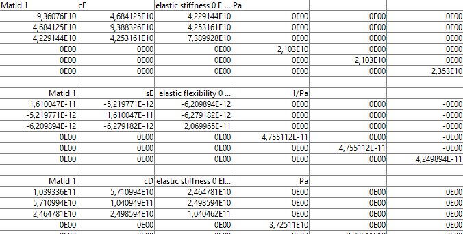
Figure 3.5: Example subset of table with the full set of mechanical, dielectric and piezoelectric coefficients in the 4 different forms of the constitutive equations
The next step (d_piezo('TutoPzPatchExt-s3')
) defines the boundary conditions and load case. We consider here two cases, the first one where the patch is free to expand, and the second one where it is mechanically constrained (all mechanical degrees of freedom are equal to 0).
In d_piezo('TutoPzPatchExt-s4')
, we can look at the deformed shape, and plot the electric field for both cases.
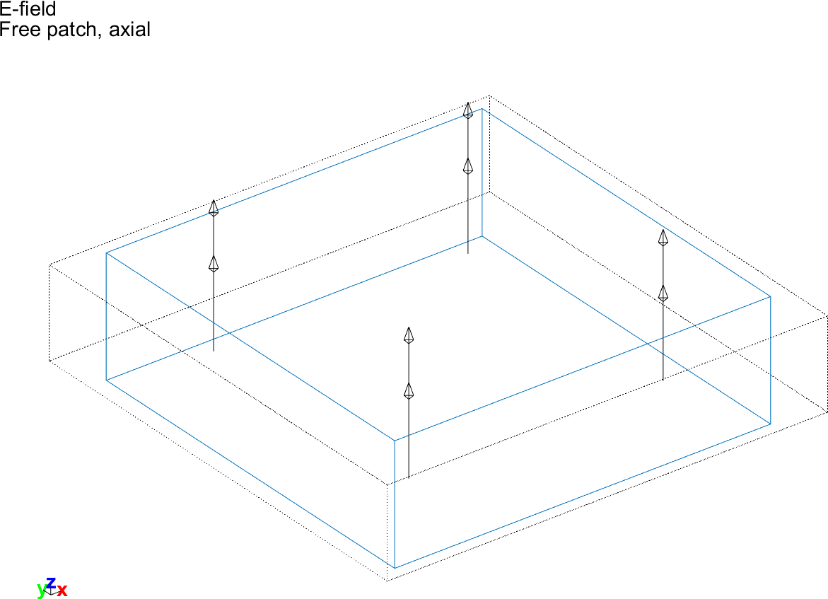
Figure 3.6: Visualization of the electric field and deformed shape for the free patch under unit voltage excitation
For the free patch deformed shape, we compute the mean strains from which d31, d32 and d33 are deduced. The values are found to be equal to the analytical values used in the model.
Relation between mean strain on free structure and d_3i
    {'E3 mean'}    {[500.0000]}    {[500]}    {'E3 analytic'}

    {'Sx'}    {[-1.8000e-10]}    {[-1.8000e-10]}    {'d_31'}
    {'Sy'}    {[-1.8000e-10]}    {[-1.8000e-10]}    {'d_32'}
    {'Sz'}    {[ 4.0000e-10]}    {[ 4.0000e-10]}    {'d_33'}
Note that the parameters of the constitutive equations can be recovered using
d_piezo('TutoPzPatchExt-s5')
.
%% Step 5 : check constitutive law
% Decompose constitutive law
CC=p_piezo('viewdd -struct',cf); %
where the fields of CC are self-explanatory. The parameters which are not directly defined are computed from the equations presented in section 2.1.
For the constrained patch, we compute the mean stress from which we can compute the e31, e32 and e33 values which are found to be equal to the analytical values used in the model.
Relation between mean stress on pure electric and e_3i
    {'Tx'}    {[-8.3642]}    {[-8.3642]}    {'e_31'}
    {'Ty'}    {[-8.3178]}    {[-8.3178]}    {'e_32'}
    {'Tz'}    {[14.2916]}    {[14.2916]}    {'e_33'}
In d_piezo('TutoPzPatch-s6')
, we can also compute the charge and the charge density (in pC/m2) accumulated on the electrodes, and compare with the analytical values
    {0x0 double              }      {'Top'       }    {'Bottom'     }
    {'Free patch, axial'     }      {[7.7473e-10]}    {[-7.7473e-10]}
    {'Constrained patch, axial'}    {[3.3876e-10]}    {[-3.3876e-10]}

Theoretical values of capacitance
    {'CT'}    {[7.7473e-10]}
    {'CS'}    {[3.3876e-10]}
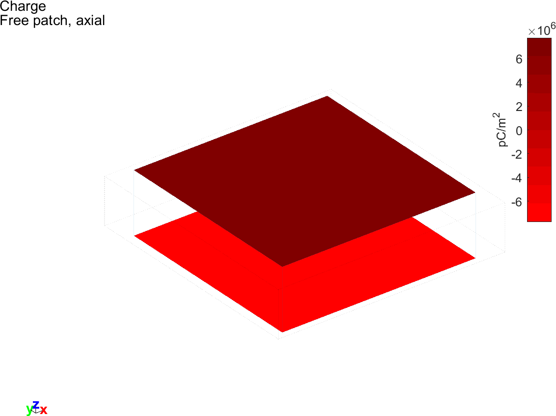
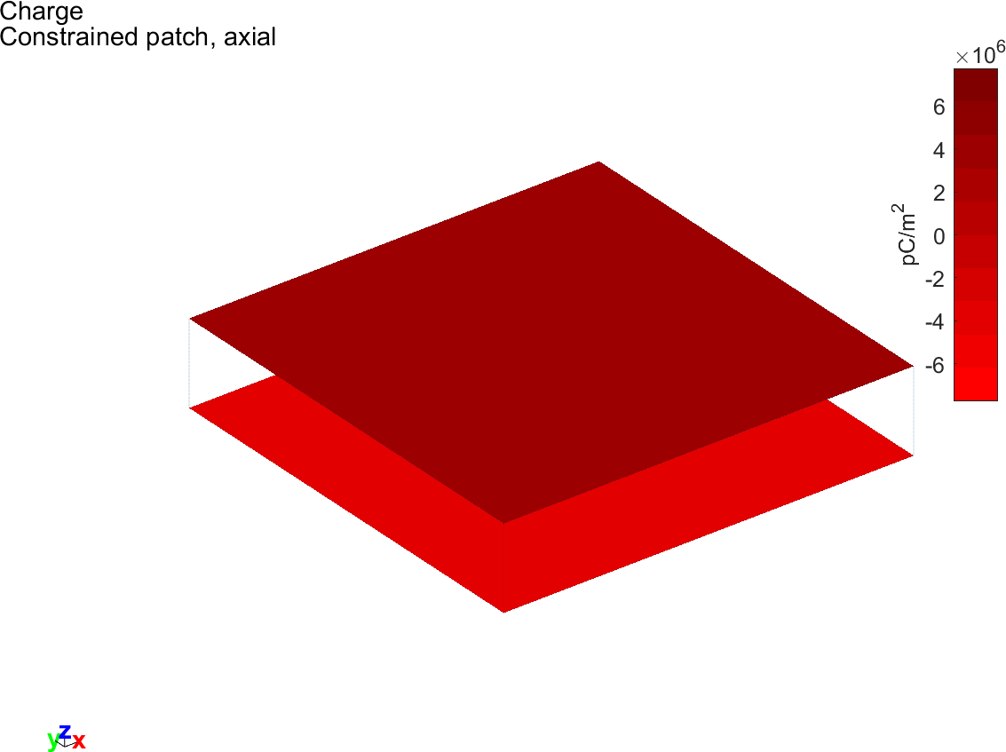
Figure 3.7: Vizualisation of the total charge on the electrodes for the unconstrained and constrained patch under unit voltage excitation
The results clearly show the very large difference of charge density between the two cases (free patch or constrained patch).
For this simple static example, a finer mesh can be used, but it does not lead to more accurate results (this can be done by changing the values in the call to d_piezo('mesh') for example:
% Build mesh with refinement
model=d_piezo('MeshPatch lx=1e-2 ly=1e-2 h=2e-3 nx=5 ny=5 nz=2');
% Now a model with quadratic elements
model=d_piezo('MeshPatch lx=1e-2 ly=1e-2 h=2e-3 Quad');
As for the patch in extension, as the fields are also uniform (see section 2.4.2), the problem can be modelled with a single 8-node element. In d_piezo('TutoPzPatchShear-s1')
, the patch is meshed and then the poling is aligned with the −y axis by performing a rotation of 90o around the x-axis .
In d_piezo('TutoPzPatchShear-s2')
and d_piezo('TutoPzPatchShear-s3')
, the response is computed both for the free case and the fully constrained case. The deformed shape for the free case is shown in Figure 3.8 together with the applied electric field:
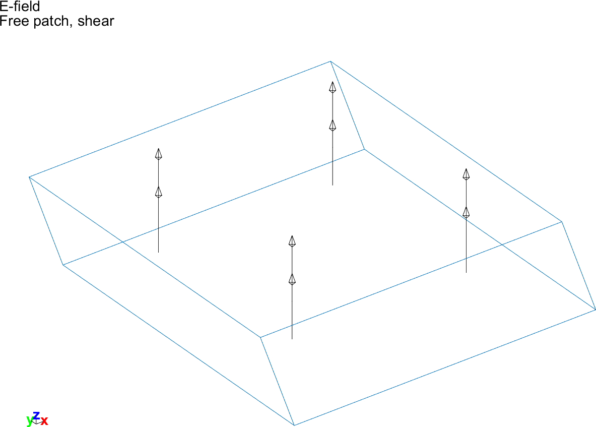
Figure 3.8: Deformed shape of a piezoelectric patch poled in the plane with an electric field applied in the out-of-plane direction
In d_piezo('TutoPzPatchShear-s4')
, the mean of shear strain and stress is evaluated and compared to the d24 and e24 piezo coefficients.
Note that the mean values are computed in the global yz axis for which a negative strain corresponds to a positive strain in the local 23 axis.
 Relation between mean strain on free structure and d_24
    {'E3 mean'}    {[500]}    {[500]}    {'E3 analytic'}
    {'Syz'}    {[5.6000e-10]}    {[5.6000e-10]}    {'d_24'}

    Relation between mean stress on pure electric and e_24
    {'Tyz'}    {[10.7234]}    {[10.7234]}    {'e_24'}
Finally in d_piezo('TutoPzPatchShear-s5')
, the capacitance is evaluated and compared to the theoretical values, showing a perfect agreement, and demonstrating the difference with the extension case for CS.
 {0x0 double              }      {'Top'       }    {'Bottom'     }
    {'Free patch, shear'     }      {[8.1900e-10]}    {[-8.1900e-10]}
    {'Constrained patch, shear'}    {[5.1874e-10]}    {[-5.1874e-10]}

Theoretical values of capacitance
    {'CT'}    {[8.1900e-10]}
    {'CS'}    {[5.1874e-10]}

