PDF Index
| SDT-piezo
Contents
Functions
PDF Index |
Other types of loads, such as surface or volumic loads are handled by the fe_load command (sdtweb('fe_load') for more details) in SDT. The case of imposed displacement is handled with fe_case('DofSet') calls.
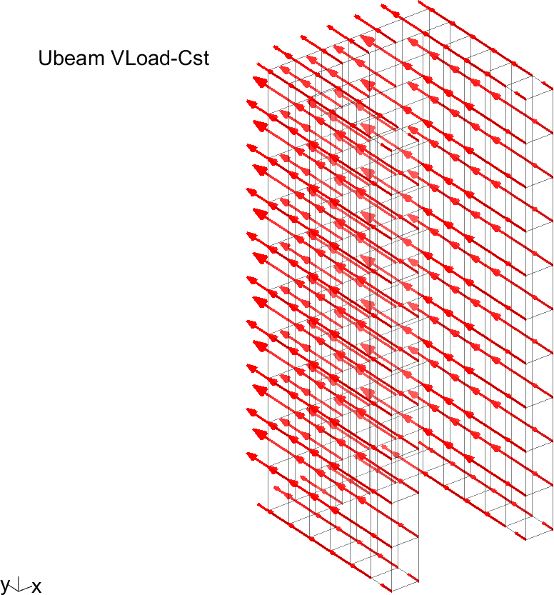
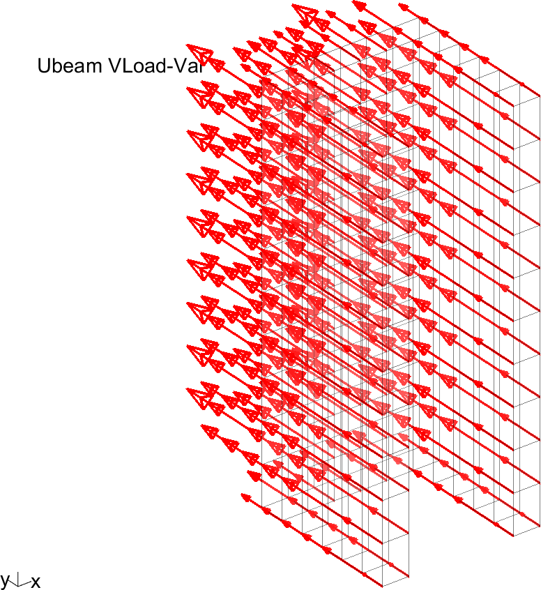
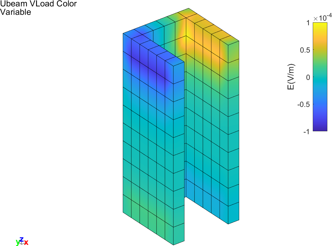
The following script illustrates the use of volume and surface loads on the U-beam.
In  d_piezo('TutoPzBeamSurfVol-s1')
, the first load is defined by 'data' and is a constant volumic load in the y-direction. The second load, defined by 'data2' is in the z-direction and its magnitude depends both on the x and z position in the U-beam (f(x,z)=x*(z−1)3). The two loads are represented in Figures 4.12 and 4.13 using arrows and color codes (for the variable force only).
d_piezo('TutoPzBeamSurfVol-s1')
, the first load is defined by 'data' and is a constant volumic load in the y-direction. The second load, defined by 'data2' is in the z-direction and its magnitude depends both on the x and z position in the U-beam (f(x,z)=x*(z−1)3). The two loads are represented in Figures 4.12 and 4.13 using arrows and color codes (for the variable force only).
%% Step 1 Apply  a volumic load and represent
model = femesh('testubeam');
data=struct('sel','groupall','dir',[0 32 0]);
data2=struct('sel','groupall','dir',{{0,0,'(z-1).^3.*x'}});
model=fe_case(model,'FVol','Constant',data, ...
                     'FVol','Variable',data2);

% Visualize loads
cf=feplot(model); iimouse('resetview');

% Make mesh transparent :
fecom('showfialpha') %

% Visualize Load
fecom proviewon

% Improve figure
sdth.urn('Tab(Cases,Constant){deflen,.5,arProp,"linewidth,2"}',cf)
fecom curtabcases 'Constant' % Shows the case 'Constant'
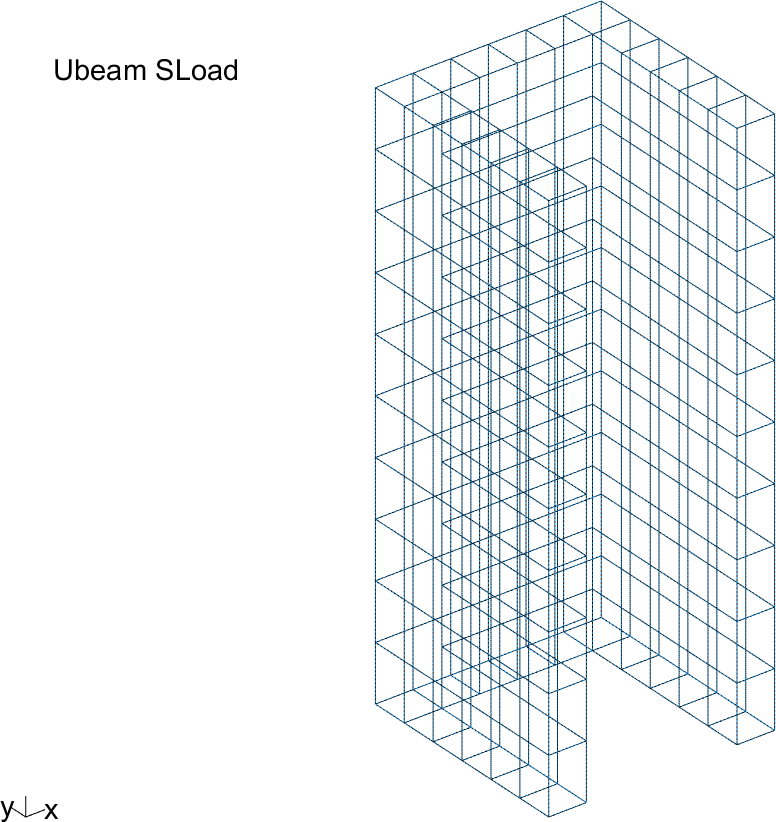
In d_piezo('TutoPzBeamSurfVol-s2')
, the surface load is defined using selectors to define the area of the surface where the load is applied. In this case, the load is on the surface corresponding to x=−0.5 and z>1.25. The resulting surface load is represented in Figure 4.14.
%% Step 2 :  Apply a surface load case in a model using selectors
data=struct('sel','x==-.5', ...
             'eltsel','withnode {z>1.25}','def',1,'DOF',.19);
model=fe_case(model,'Fsurf','Surface load',data); cf=feplot(model);
In d_piezo('TutoPzBeamSurfVol-s3')
, the same is done using node lists.
%% Step 3 : Applying a surfacing load case in a model using node lists
data=struct('eltsel','withnode {z>1.25}','def',1,'DOF',.19);
NodeList=feutil('findnode x==-.5',model);
data.sel={'','NodeId','==',NodeList};
model=fe_case(model,'Fsurf','Surface load 2',data); cf=feplot(model);
And lastly in d_piezo('TutoPzBeamSurfVol-s4')
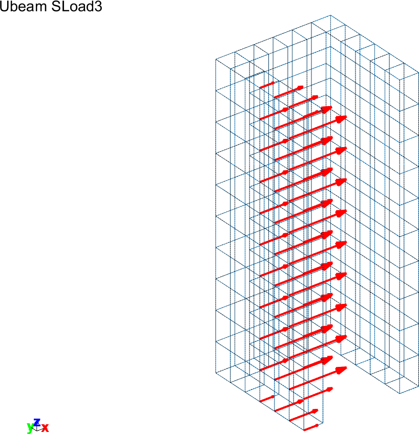
, the use of sets to define surface loads (Figure 4.15) is illustrated.
%% Step 4 : Applying a surfacing load case in a model using sets

% Define a face set
[eltid,model.Elt]=feutil('eltidfix;',model);
i1=feutil('findelt withnode {x==-.5 & y<0}',model);i1=eltid(i1);
i1(:,2)=2; % fourth face is loaded
data=struct('ID',1,'data',i1,'type','FaceId');
model=stack_set(model,'set','Face 1',data);

% define a load on face 1
data=struct('set','Face 1','def',1,'DOF',.19);
model=fe_case(model,'Fsurf','Surface load 3',data); cf=feplot(model);
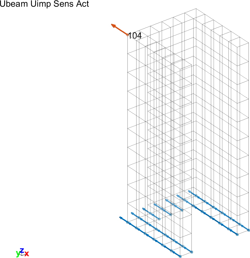
Another type of load is the case when degrees of freedom are imposed (imposed displacement, velocity, acceleration, or electric potential in the case of piezoelectric actuators). The script below illustrates the case where the U-beam has an imposed displacement on the cantilever side, in the y-direction (Figure 4.16).
In d_piezo('TutoPzBeamUimp-s1')
, the mesh is created and the boundary conditions are applied. One has to be careful not to block the degrees of freedom in the direction of the imposed motion (y in this example):
%% Step 1 Meshing and BC
model = femesh('test ubeam');
% BC : Impose displacement -  Fix all other dofs for Base
model=fe_case(model,'FixDof','Clamping','z==0 -DOF 1 3');
In d_piezo('TutoPzBeamUimp-s2')
, the displacement at the base is imposed using a 'DofSet' entry.
%% Step 2 Apply base displacement in y-direction
% find node z==0
nd=feutil('find node z==0',model);
data.DOF=nd+.02; data.def=ones(length(nd),1);
model=fe_case(model,'DofSet','Uimp',data);
Then in In d_piezo('TutoPzBeamUimp-s3')
, a point sensor is introduced on node 104 in direction y (Figure 4.16).
Finally in (d_piezo('TutoPzBeamUimp-s4')
),
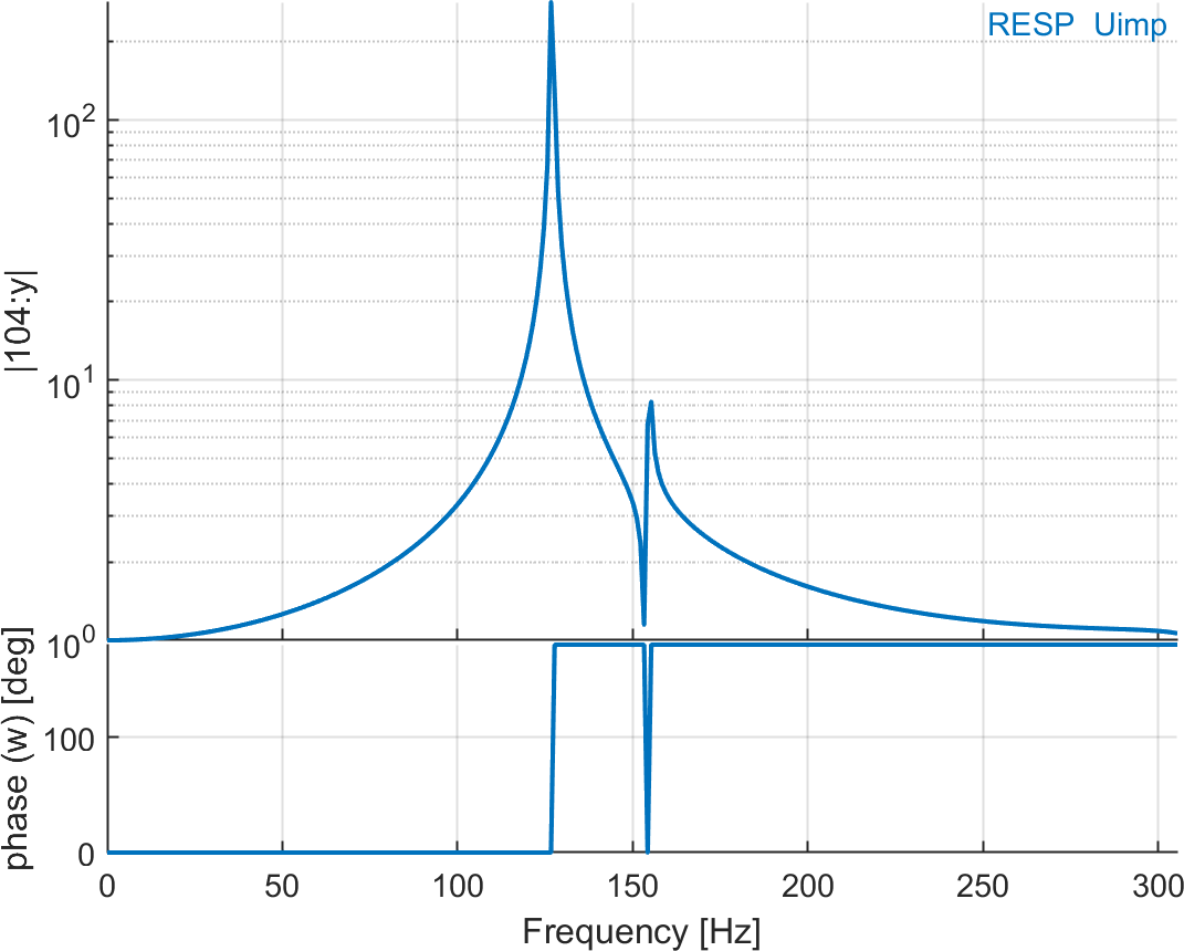
the transfer function is computed using fe_simul and plotted in the iiplot environment (Figure 4.17).
As expected, the static response is unitary, as the U-beam does not deform when a uniform unitary displacement of the base is imposed, so that node 104 moves in the same direction and with the same magnitude as the base.
Note that it is also possible to impose an acceleration when building state-space models, which will be detailed in section 6.3.