PDF Index
| SDT-base
Contents
Functions
PDF Index |
Three kinds of manipulations are possible using the feplot GUI
feplot figures are used to view FE models and hold all the data needed to run simulations. Data in the model can be viewed in the property figure (see section 4.4.4). Data in the figure can be accessed from the command line through pointers as detailed in section 4.4.3. The feplot help gives architecture information, while fecomlists available commands. Most demonstrations linked to finite element modeling (see section 1.2 for a list) give examples of how to use feplot and fecom.
The first step of most analyzes is to display a model in the main feplot figure. Examples of possible commands are (see fecom load for more details)
As an example, you can load the data from the gartfe demo, get cf a SDT handle for a feplot figure, set the model for this figure and get the standard 3D view of the structure
 model=demosdt('demogartfe')
 cf=feplot;       % open FEPLOT and define a pointer CF to the figure
 cf.model=model;
The main capabilities the feplot figure are accessible using the figure toolbar, the keyboard shortcuts, the right mouse button (to open context menus) and the menus.
List of icons used in GUIs
 | Model properties used to edit the properties of your model. |
 | Start/stop animation |
 | Previous Channel/Deformation |
 | Next Channel/Deformation |
 | iimouse zoom |
 | Orbit. Remaining icons are part of MATLAB cameratoolbar functionality. |
 | Snapshot. See iicom ImWrite. |
The contextmenu associated with your plot may be opened using the right mouse button and select Cursor. See how the cursor allows you to know node numbers and positions. Use the left mouse button to get more info on the current node (when you have more than one object, the n key is used to go to the next object). Use the right button to exit the cursor mode.
Notice the other things you can do with the ContextMenu (associated with the figure, the axes and objects). A few important functionalities and the associated commands are
The figure Feplot menu gives you access to the following commands (accessible by fecom)
You can typically view stack entries by clicking on the associated entry and using ProViewOn ( icon). Handling of which deformation is shown in multi-channel entries is illustrated below
 model=demosdt('demo UbeamDofLoad');cf=feplot;
 sdth.urn('Tab(Cases,Point.*1){Proview,on}',cf)

 % Control channel in multi column DOFLoad
 cf.CStack{'Point load 1'}.Sel.ch=2;fecom('proViewOn');
cf1=feplot returns a pointer to the current feplot figure. The handle is used to provide simplified calling formats for data initialization and text information on the current configuration. You can create more than one feplot figure with cf=feplot(FigHandle). If many feplot figures are open, one can define the target giving an feplot figure handle cf as a first argument to fecom commands.
The model is stored in a graphical object. cf.model is a method that calls fecom InitModel. cf1.mdl is a method that returns a pointer to the model. Modifications to the pointer are reflected to the data stored in the figure. However mo1=cf.mdl;mo1=model makes a copy of the variable model into a new variable mo1.
cf.Stack gives access to the model stack as would cf.mdl.Stack but allows text based access. Thus cf.Stack{'EigOpt'} searches for a name with that entry and returns an empty matrix if it does not exist. If the entry may not exist a type must be given, for example cf.Stack{'info','EigOpt'}=[5 10 1].
cf.CStack gives access to the case stack as would calls of the form
Case=fe_case(cf.mdl,'getcase');stack_get(Case,'FixDof','base') but it allows more convenient string based selection of the entries.
cf.Stack and cf.CStack allow regular expressions text based access. First character of such a text is then #. One can for example access to all of the stack entries beginning by the string test with cf.Stack{'#test.*'}. Regular expressions used by SDT are standard regular expressions of Matlab. For example . replaces any character, * indicates 0 to any number repetitions of previous character...
Finite element models are described by a data structures with the following main fields (for a full list of possible fields see section 7.6)
| .Node | nodes |
| .Elt | elements |
| .pl | material properties |
| .il | element properties |
| .Stack | stack of entries containing additional information cases (boundary conditions, loads, etc.), material names, etc. |
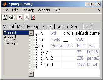
The model content can be viewed using the feplot property figure. This figure is opened using the icon, or fecom('ProInit').
This figure has the following tabs
mode, associated elements in selection are shown. See section 4.5.1.
The figure icons have the following uses
| | Model properties used to edit the properties of your model. |
| Active display of current group, material, element property, stack or case entry. Activate with fecom('ProViewOn'); |
 | Open the iiplot GUI. |
 | Open/close feplot figure |
 | Refresh the display, when the model has been modified from script. |
This section describes functionality accessible with the Edit list item in the Model tab. To force display use sdth.urn('feplot.Tab(Model,Edit)').
Below are sample commands to run the functionality from the command line.
model=demosdt('demoubeam');cf=feplot;
sdth.urn('feplot.Tab(Model,Edit)')
fecom(cf,'addnode')
fecom(cf,'addnodecg')
fecom(cf,'addnodeOnEdge')
fecom(cf,'RemoveWithNode')
fecom(cf,'RemoveGroup')
fecom(cf,'addElt tria3')

fe_case(cf.mdl,'rbe3','RBE3',[1 97 123456 1 123 98 1 123 99]);
fe_case(cf.mdl,'rbe3 -append','RBE3',[1 100 123456 1 123 101 1 123 102]);
fecom addRbe3
feplot displays shapes and color fields at nodes. The basic def data structure provides shapes in the .def field and associates each value with a .DOF (see mdof). For other inits see fecom InitDef.
 [model,def]=demosdt('Demo gartfe'); % Get example
 cf=feplot(model,def);  % display model and shapes
 fecom('ch7');          % select channel 7 (first flex mode)
 fecom('pro');          % Show model properties
Scan through the various deformations using the +/- buttons/keys or clicking in the deformations list in the Deformations tab. From the command line you can use fecom ch commands.
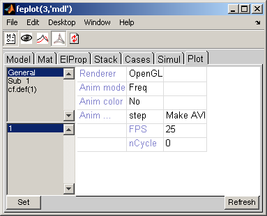
Animate the deformations by clicking on the button. Notice how you can still change the current deformation, rotate, etc. while running the animation. Animation properties can be modified with fecom Anim commands or in the General tab of the feplot properties figure.
Modeshape scaling can be modified with the l/L key, with fecom Scale commands or in the Axes tab of the feplot properties figure.
You may also want to visualize the measurement at various sensors (see section 4.7 and fe_sens) using a stick or arrow sensor visualization (fecom showsens or fecom showarrow). On such plots, you can label some or all degrees of freedom using the call fecom ('doftext',idof).
Look at the fecom reference section to see what modifications of displayed plots are available.
Modeshape superposition is an important application (see plot of section 2.8.1) which is supported by initializing deformations with the two deformation sets given sequentially and a fecom ch command declaring more than one deformation. For example you could compare two sets of deformations using
 [model,def]=demosdt('demo gartfe');cf=feplot(model); % demo init
 cf.def(1)=def;  % First set of deformations
 def.def=def.def+rand(size(def.def))/5;
 cf.def(2)=def;  % second set of deformations
 fecom('show2def'); fecom('scalematch');
where the scalematch command is used to compare deformations with unequal scaling. You could also show two deformations in the same set
 cf=demosdt('demo gartfe plot');
 fecom(';showline; ch7 10')
The -,+ buttons/commands will then increment both deformations numbers (overlay 8 and 11, etc.).
Element selections play a central role in feplot. They allow selection of a model subpart (see section 7.12) and contain color information. The following example selects some groups and defines color to be the z component of displacement or all groups with strain energy deformation (see fecom ColorData commands)
 cf=demosdt('demo gartfe plot');
 cf.sel(1)={'group4:9 & group ~=8','colordata z'};
 pause
 cf.def=fe_eig(cf.mdl,[6 20 1e3]);
 cf.sel(1)={'group all','colordata enerk'};
 fecom('colorbar');
You can also have different objects point to different selections. This model has an experimental mesh stored in element group 11 (it has EGID -1). The following commands define a selection for the FEM model (groups 1 to 10) and one for the test wire frame (it has EGID<0). The first object cf.o(1) displays selection 1 as a surface plot (ty1 with a blue edge color. The second object displays selection to with a thick red line.
 cf=demosdt('demo gartfe plot');
 cf.sel(1)={'group4:10'};  cf.sel(2)='group1:3';
 cf.o(1)={'ty1 def1 sel1','edgecolor','b'}
 cf.o(2)={'ty2sel2','edgecolor','r','linewidth',2}
Note that you can use FindNode commands to display some node numbers. For example try fecom('textnode egid<0 & y>0').
For reference information on colors, see fecom ColorData.
When preparing a model, one often needs to visualize property colors.
 cf=feplot(demosdt('demogartfe'));
 fecom('ColorDataMat'); % Display color associated with MatId
 % Now a partial selection with nicer transparency
 cf.sel={'eltname~=mass','ColorDataPro-alpha.1-edgealpha .05'}
How do I keep group colors constant when I select part of a model?
One can define different types of color for selection using fecom ColorData. In particular one can color by GroupId, by ProId or by MatId using respectively fecom colordatagroup, colordatapro or colordatamat. Without second argument, colors are attributed automatically. One can define a color map with each row of the form [ID Red Green Blue] as a second argument: fecom('colordata',colormap). All ID do not need to be present in colormap matrix (colors for missing ID are then automatically attributed). Following example defines 3 color views of the same GART model:
cf=demosdt('demo gartFE plot');
% ID Red Green Blue
r1=[(1:10)' [ones(3,1); zeros(7,1)] ...
    [zeros(3,1); ones(7,1)] zeros(10,1)]; % colormap
fecom('colordatagroup',r1) % all ID associated with color
% redefine groups 4,5 color
fecom('colordatagroup',[4 0 0 1;5 0 0 1]);
% just some ID associated with color
fecom('colordatapro',[1 1 0 0; 3 1 0 0])
Color at nodes can be based on the current display. In particular, ColorDataEvalA, EvalX, ... EvalRadZ, EvalTanZ use the information of current motion from initial position to generate a color field dynamically. The advantage of this strategy is that no prior computation is needed.
Display of specific fields is another common application. Thus ColorDataDOF 19 displays DOF .19 (pressure). This the field is not needed to display the motion of nodes, prior extraction from the deformations is needed.
Display of energies is a typical case of color at elements. Since computing energies for many deformations can take time, it is considered best practice to compute energies first and display energies next.
cf=demosdt('demo gartFE plot');
cf.def=fe_def('subdef',cf.def,cf.def.data>1);fecom('ch1');%Only keep flexible modes
% If EltId are not consistent you may need to fix them
% The ; in 'eltidfix;' is used to prevent display of warning messages
[eltid,cf.mdl.Elt]=feutil('eltidfix;',cf.mdl);
Ek=fe_stress('Enerk -curve',cf.mdl,cf.def);
fecom(cf,'ColorDataElt',Ek)          % Values for each element
% Sum by group
fecom(cf,'ColorDataElt -bygroup -frac -colorbartitle "Frac %"',Ek)
More details are given in fe_stress feplot.
feplot lets you define and save advanced views of your model, and export them as .png pictures.
What is displayed in a feplot figure is defined by a set of objects. Once you have plotted your model with cf=feplot(model), you can access to displayed objects through cf.o(i) (i is the number of the object). Each object is defined by a selection of model elements ('seli') associated to some other properties (see fecom SetObject). Selections are defined as FindElt commands through cf.sel(i). Displayed objects or selections can be removed using cf.o(i)=[] or cf.sel(i)=[].
Following example loads ubeam model, defines 2 complementary selections, and displays the second as a wire frame (ty2):
model=demosdt('demoubeam'); cf=feplot
% define visualisation
cf.sel(1)='WithoutNode{z>1 & z<1.5}';
cf.sel(2)='WithNode{z>1 & z<1.5}';
cf.o(1)={'sel1 ty1','FaceColor',[1 0 0]}; % red patch
cf.o(3)={'sel2 ty2','EdgeColor',[0 0 1]}; % blue wire frame
% reinit visualisation :
cf.sel(1)='groupall';
cf.sel(2)=[]; cf.o(3)=[];
There is no theoretical size limitation for models to be displayed. However, due to the use of Matlab figures, and although optimization efforts have been done, feplot can be very slow for large models. This is due to the inefficient use of triangle strips by the Matlab calls to OpenGL, but to ensure robustness SDT still sticks to strict Matlab functionality for GUI operation.
When encountering problems, you should first check that you have an appropriate graphics card, that has a large memory and supports OpenGL and that the Renderer is set to opengl. Note also that any X window forwarding (remote terminal) can result in very slow operation: large models should be viewed locally since Matlab does not support an optimized remote client.
To increase fluidity it is possible to reduce the number of displayed patches using fecom command SelReducerp where rp is the ratio of patches to be kept. Adjusting rp, fluidity can be significantly improved with minor visual quality loss.
Following example draws a 50x50 patch, and uses fecom('ReduceSel') to keep only a patch out of 10:
model=feutil('ObjectQuad',[-1 -1 0;-1 1 0;1 1 0;1 -1 0],50,50);
cf=feplot(model); fecom(cf,'showpatch');
fecom(cf,'SelReduce .1'); % keep only 10% of patches.
If you encounter memory problems with feplot consider using fecom load-hdf.
You should not save feplot figures but models using fecom Save.
To save images shown in feplot, you should see iicom ImWrite. If using the MATLAB print, you should use the -noui switch so that the GUI is not printed. Example print -noui -depsc2 FileName.eps.
When using fecom ColorDataEval commands (useful when displayed deformation is restituted from reduced deformation at each step), color scaling is updated at each step.
One can use fecom('ScaleColorOne') to force the colorbar scale to remain constant. In that case one can define the limit of the color map with set(cf.ga,'clim',[-1 1]) where cf is a pointer to target feplot figure, and -1 1 can be replaced by color map boundaries.
Several strategies are available depending on the user needs.
convert('AnimMovie25') will generate a 25 steps feplot animation as an animated gif.
To pilot a subsampling of steps, see fecom Anim.
Note that the convert function is a gateway function to the convert function of ImageMagick, that should be installed on your system. You can look up https://www.imagemagick.org for more information.
writerObj = VideoWriter(['TEST2_ANIM.avi']); %'Archival');
 writerObj.FrameRate=830; % fps
 writerObj.Quality=100;
 open(writerObj);
 cf.ua.PostFcn=sprintf(['evalin(''base'','...
'''frame = getframe(gcf);writeVideo(writerObj,frame);'')']);
 frame = getframe;
 writeVideo(writerObj,frame); % frame will contain the film
 close(writerObj);