PDF Index
| SDT-rotor
Contents
Functions
PDF Index |
The SDT/Rotor toolbox supports analysis of 1D models of symmetric rotors composed of
You can generate a beam model of your rotor by providing a skyline (points not on the axis defining the radius at various locations). Use NaN to define 2 segments. See rotor1d Skyline for more details.
xy=[0 0; 0 .1;1 .1;1 1;1.1 1;1.1 .1;2 .1];
xy(:,3)=0;  figure(1);plot(xy(:,1),xy(:,2));
% Mesh as beams
mo1d=rotor1d('skylineToBeam',xy);
% Add bearings as spring elements:
mo1d=rotor1d('AddBearing DOF -123 k 1e4 -keep',mo1d,[0.1 0 0]);
mo1d=rotor1d('AddBearing DOF -123 k 1e4 -keep',mo1d,[1.9 0 0]);

% now view as 3D model
mo2d=rotor1d('1To2d lc 5e-2',mo1d);
cf=feplot;cf.model=rotor2d('buildFrom2D nsec16',mo2d);
You can also add beam through rotor1d Addbeam command.
mo1d=rotor1d('AddBeam x1 0 x2 0.7 r2 0.77 MatID 1',[]); % add rod
mo1d=rotor1d('AddBeam x1 0.5 x2 0.8 r1 0.77 r2 0.90 MatID 1',mo1d); %add tube
mo2d=rotor1d('1To2d lc 5e-2',mo1d);
cf=feplot; cf.model=mo2d; fecom colordatapro;
For 2D rotor representations, the SkyLineTo2d command eases the generation of simple rotors. Note how in the following example Nan separators are used to generate a rotor in multiple parts : center shaft first, then after the separator various disks.
xy=[ 0 0;0  0.00945;0.0088  0.00945; 0.0088  0.0057;
0.042  0.0057;0.042  0.00938; 0.057  0.00938;
0.057  0.008;0.0637  0.008; 0.0637  0.00595;
0.0919  0.00595;0.0919  0.00925; 0.0979  0.00925;
0.0979  0.006;0.121  0.006; 0.121  0.008;
0.127  0.008;0.127  0.0095; 0.142  0.0095;
0.142  0.006;0.175  0.00565; 0.226  0.00565; 0.226  0.0088;
0.232  0.0088;
NaN 0.0057; % Disk
0.00952  0.0057;0.00952  0.008;
 0.0209  0.008; 0.0209  0.0369;
 0.0242  0.0369; 0.0242  0.0572; 0.0266  0.0572;0.0266  0.0369;
 0.0299  0.0369; 0.0299  0.008;0.0413 0.008
NaN .00565; % Separator giving non zero internal diameter .00565
0.177+.01  0.0057;0.177+.01  0.02;0.191  0.02; 0.191  0.0057;
NaN .00565; % Separator giving non zero internal diameter .00565
0.197+.005  0.0374; 0.215-.005  0.0374;  % Impeller
 0.215-.005  0.006+.003;0.222-.002  0.006+.003; % between sub disks
 0.222-.002  0.0775; 0.2259  0.0775;
];
xy(:,3)=0;
mo2d=rotor1d('skyline To2d -lc .005',xy); % x axis
mo2d.pl=[ ...
   1 fe_mat('m_elastic',1,1)  200000000000 0.29 7800
   2 fe_mat('m_elastic',1,1)  7.17e10 0.33 2830 %2830
   3 fe_mat('m_elastic',1,1)  3.07e12 0.3 .78 % 7800
];
mo2d.Elt(feutil('findelt matid 2 3 4 5',mo2d),5:6)=2;
mo2d.Elt(feutil('findelt innode {x>=.15 & y<=.0057}',mo2d),5:6)=3;
mo2d.Elt(feutil('findelt innode {x>=.22 & y<=.01}',mo2d),5:6)=3;
feplot(mo2d); fecom colordatamat

cf=feplot;cf.model=rotor2d('buildFrom2D nsec16',mo2d);
cf.sel={'-disk1','ColorDataMat'};fecom(';view1')
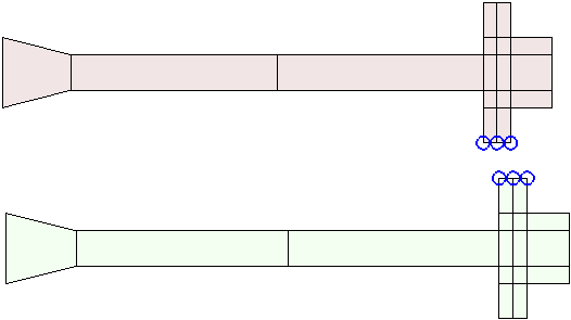
Following example builds by hand a simple 1D rotor, with one shaft, one disk and 2 bearing stifnesses. It is almost the same as one accessible through d_rotor TestShaftDiskMdl.
 % define mesh :
 model=struct('Node', ...
         [1 0 0 0  0 0 0; 2 0 0 0  0.4/3 0 0;
          3 0 0 0  0.4*2/3 0 0; 4 0 0 0  0.4 0 0]);
 model.Elt=feutil('ObjectBeamLine',(1:4)'); % define shaft
 model.Elt=feutil('ObjectMass',model,2,...
     [16.5 16.5 16.5 0.18608 0.093 0.093]); % add disk
 model=feutil('AddElt',model,'celas', ...
      [3 0 2 0 100 0 0; 3 0 3 0 101 0 0]); % add bearings (y and z stifness)
 % define properties
 model.pl=m_elastic('dbval 1 steel');  % shaft material
 model.il=p_beam('dbval 1 circle 1e-2'); % shaft, r=1e-2
 model.il=p_spring(model.il,'dbval 100 5e5','dbval 101 5e5'); % bearings
 % ends boundaries :
 model=fe_case(model,'fixdof','Ends',...
     [1.01;1.02;1.03;4.01;4.02;4.03]);
 % Assemble nominal matrices:
 model=fe_caseg('assemble -reset -secdof -matdes 2 1 70',model);
 cf=feplot(model);
 % For solution see sdtweb('freqstud')
Note that at this time only fixed frame representation is available for such 1d rotors (beam1 and mass1 elements). Gyroscopic coupling is then computed under MatType 70 ( The formula for gyroscopic coupling can be found in [6]) The nominal representation for these models is then the Eulerian point of view where the displacement of the rotor is expressed in a non-rotating frame. For the 1D representation, the model nodes are always placed on the nominal rotation axis. Thermal and pre-stress effects are not accounted for.
The rotor module supports all 3D elements of SDT. 2D models are only considered through an extrusion and 3D cyclic symmetry. One can import a volume model, or mesh it using feutil meshing commands. This section describes procedures to mesh volumes from 1D and 2D models.
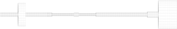
From 1D rotor model meshed using beam1 elements, one can create a 2D model using rotor1d 1To3D command. Note that mass1 elements can not be converted for the moment. For example, with section ?? rotor model
xy=[0 0; 0 .1;1 .1;1 1;1.1 1;1.1 .1;2 .1];
mo1d=rotor1d('skyline ToBeam',xy); % Mesh as beams
% Add bearings as spring elements:
mo1d=rotor1d('AddBearing DOF -123 k 1e4 -keep',mo1d,[0.1 0 0]);
mo1d=rotor1d('AddBearing DOF -123 k 1e4 -keep',mo1d,[1.9 0 0]);
mdl3d=rotor1d('1To3d-quad-lc0.02-div24',mo1d); % build 3d rotor
cf=feplot(mdl3d)
Command option -quad force the use of quadratic elements (hexa20) instead of linear elements (hexa8).
Shaft is meshed using hexa8 degenerated elements. The edges on the axis of the shaft are using the same nodes as the beam nodes so that bearings described by celas in 1D intial rotor can remain the same. RBE3 rings are created at each bearing celas. Concentrated masses (no inertia) on the axis are also left.
THIS IS NO LONGER TRUE BUT SHOULD BE REACTIVATED XXX: mass1 elements with inertia that represents disks, are meshed as volume disks of arbitrary thickness (dt) 0.005, with radius R2 computed so that inertia along rotation axis is the same (Ir=0.5m(R22+R12)) and then density is computed to match the mass m (m=(R22−R12)*dt). (R1 is shaft radius). Young modulus of disk is taken at 100*steel modulus.
Gyroscopic coupling and centrifugal stifness for 3D elements are only described in the rotating frame, that is to say under MatType 7 and MatType 8.
 mdl3d=fe_mat('defaultil',mdl3d); % default element pro
 mdl3d=fe_mat('defaultpl',mdl3d); % default material pro
 % Assemble nominal matrices:
 mdl3d=fe_caseg('assemble -reset -secdof -matdes 2 1 7 8',mdl3d);
One can also find an example of a 3D rotor in d_rotor('TestVolShaftDiskMdl').
  data={'Rs'  ,0.01  , 'shaft radius';
        'Rd'  ,0.15  , 'disk radius';
        'Ls'  ,0.4   , 'shaft length';
        'Ld'  ,0.03,   'disk thickness';
        'yd'  ,0.4/3,  'disk position on the shaft'
        'yb'  ,0.4*2/3,'bearing stifness position on the shaft'
        'Tol' ,0.05,   'elt length Tol'
        };
  model=d_rotor('TestVolShaftDiskMdl',data);
rotor2d BuildFrom2D convert 2d model to 3d model using cyclic symetry. For example, to convert previous 2D model:
mdl2d=rotor1d('1To2d-quad-lc0.02',mo1d);
mdl3d=rotor2d('buildFrom2D -close nsec3 div8',mdl2d);
The SDT fe_cyclic function only handles single sector models using symmetry conditions. SDT/Rotor extends the capabilities by dealing with a full (possibly multi-stage, then called shaft) rotor model.
Building a disk/shaft model is done in two steps. For each sector, one defines matching edges using a fe_cyclic Build command, the generates a disk/shaft model using fe_cyclicb DiskFromSector.
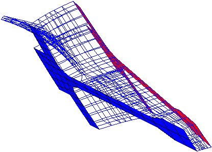
demosdt(['download-back donnees_secteur.dat'])% xxx missing patchfile
% -removeface : removes skin elements
samcef('read-removeface',fullfile(sdtdef('tempdir'),'donnees_secteur.dat'));
cf=feplot;
% Fix sector edges
fe_cyclic('buildepsl .1 fix',cf.mdl);
fecom('curtabCases','Symmetry')
fecom(';view3;proViewOn');
The left and right edges of sectors should be conform ! Practically you need to mesh the two surfaces first (possibly generate the second by rotation of the first). Then mesh the interior. You will note that this typically requires at least two layers of element for tetra10 meshing.
Typically blades have an angle with respect to the er,ez plane. In a number of cases, removing this angle makes node and element selection easier. With two nodes the FixTheta command modifies node positions by removing the angle. The transformation is saved in info,FixTheta stack entry and the back transformation is obtained using a FixTheta call with no argument.
 cf=feplot(2);cf=d_rotor('TestSector');%sdtweb('d_rotor.m#TestSector')
 n1=cf.mdl.Node; % save nodes

 cg=feplot(5); % place rectified model in figure(5)
 cg.mdl=fe_cyclicb('MeshFixTheta 10061 10086 -offset 80',cf.mdl);
 fecom(cg,'view2')
 % verify that the back step works
 cf.mdl=fe_cyclicb('MeshFixTheta',cg.mdl);fecom(cf,'view1')
 if norm(cf.mdl.Node-n1)>1e-10; error('Back transform failed');end
In multi-stage cyclic symmetry, each stage is modeled using a superelement called diski (see fe_cyclicb DiskFromSector). Coupling between stages is done using elements. The most consistent approach is to use a physical area that is properly meshed for the full 360 degrees, but this may be difficult in particular when the mesh refinement is notably different between the two stages, so that a node to surface penalized connection is also implemented and an example given at the end of this section.
Two steps are required:
Note that fe_shapeoptim can be used to local deform the disk in order to allow rim meshing.
 % load two disk example with space between disks
 cf=demo_cyclic('TestForMeshRimVol')

 % RimStep1: select nodes at the matching interfaces
 fe_cyclicb('DisplayAllEdges',cf);
 % start cursor to pick values : fe_fmesh('3dlineinit')
 n1=[12 18 24 1127 1133 1139];

 % RimStep2: build rims and tessellate
 fe_cyclicb('MeshRimStep2 epsl.1',cf,n1);
 cf.sel='EltName~=SE';fecom('showpatch');
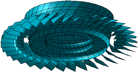
If you choose the penalty approach here is a working example where the edges of sector edges are assumed coincident thus allowing an automated search of intersection with the -FindIntersect option.
 % load two disk example with space between disks
 cf=demo_cyclic('testrotor 7 10 3 -NoRim -RimH .1 -blade -cf 2 reset');

 % RimStep1: find nodes at the matching interfaces
 n1=fe_cyclicb('DisplayAllEdges -FindIntersect epsl .2',cf);

 % RimStep2: build rims as springs
fe_cyclicb('MeshRimStep2 epsl.1 -kp 1e12 -slavedisk 1 3 -masterdisk 2',cf,n1);

cf.sel={'groupall','colordatagroup -edgealpha .05 -alpha.1'}
 def=fe_cyclicb('shaft eig 0',cf.mdl);
sel={'disk1','groupall';'disk2','groupall';'disk3','groupall';'rim',''};
 cf.def=fe_cyclicb('DisplaySel',cf,def,sel);
fecom('ColorDataEvalTanz')
Meshing tools also include procedures to build viewing meshes from the finite element mesh. fe_cyclicb('MeshRimLine2Patch',cf,sel) aims to build viewing meshes made of surface elements connecting selected nodes of the true mesh of the rotor. sel can be:
The selection is stored in the cf.mdl.Stack{'info','ViewMesh'}. If the -reset option is not specified, the current selection is appended to the existing one. For each project, you should typically edit a script similar to the following
 cf=demo_cyclic('BuildStep0');

 % Viewing mesh step 1: disk elements
 fe_cyclicb('DisplayAllEdges',cf);
 %fe_fmesh('3dLineInit',cf); % right click 'Type' or 'Done'
 L=[1 3 5 15 26 0 1121 1123 1125 1135 1146 0 13 15 18 1133 1135 1138];
 fe_cyclicb('MeshRimLine2Patch -reset',cf,L);

 % Viewing mesh step 2: blade elements
 % disk1
 fe_cyclicb('DisplayFirst',cf,{'disk1'});
 %fe_fmesh('3dLineInitAddInfo Quad4',cf); % pick four nodes to form a quad
 % use right click 'Type' or 'Done' to display
 Elt=[Inf abs('quad4');
 154 156 152 148 1 1;148 146 150 154 1 1;
 146 142 144 150 1 1;142 111 83 144 1 1];
 fe_cyclicb('MeshRimLine2Patch',cf,Elt);

 % disk2
 fe_cyclicb('DisplayFirst',cf,{'disk2'});
 fe_fmesh('3dLineInitAddInfo Quad4',cf); % pick four nodes to form a quad
 model.Elt=[Inf abs('quad4');
 1274 1276 1272 1270 1 1;1270 1272 1268 1266 1 1
 1266 1268 1264 1262 1 1;1262 1231 1203 1264 1 1];
 fe_cyclicb('MeshRimLine2Patch',cf,model.Elt);
 fecom('ShowPatch');
 % save cf.Stack{'info','ViewMesh'}

 % Once the geometry generated typical calls are
 fesuper('Sebuildsel -initrot',cf,cf.Stack{'info','ViewMesh'})
 fe_cyclicb('Displaysel 2',cf,def,cf.Stack{'info','ViewMesh'})