1D models

SDT-rotor Contents Functions

4.3 1D models

4.3.1 1D example in a fixed frame

This first example treats the simple case, taken from [6], of a shaft with a rotating disk at one third the length.

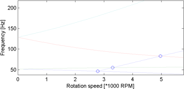
In order to compare this model to the simple 2 DOF model of Lalanne (see section 4.2) we project the matrices on the 2 sin shape function of the shaft. Relative error for mass matrix is 0.01%, 4.59% for stiffness and 1.64% for gyroscopic matrix. Campbell for the projected model and the Lalanne 2 DOF model are almost the same. For the full 1d model (not projected) the increasing of the frequency of 1rst forward whirl mode tends to an asymptote.

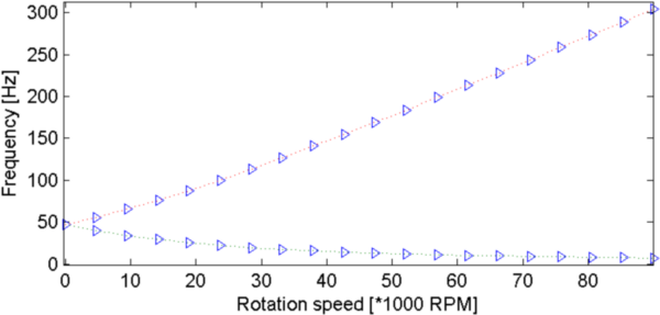
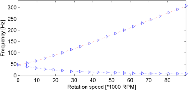
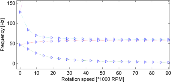
Figure 4.9: Campbell diagrams. Left: 1D rotor (up: projected on 2 DOF, down: full model), right: Lalanne 2 DOF rotor.

Following example performs preceding comparison :

% - LALANNE 2DOF
model2DOF=[]; m=14.29; k=1.195e6; a=2.871; 
kxx=0; kzz=0; kxz=0; kzx=0;% bearing
% define model matrices :
model2DOF.K={m*eye(2), k*eye(2)+sin(pi*2/3)^2*[kxx kxz;kzx kzz],a*[0 -1;1 0]};
model2DOF.DOF=1+[.01;.03];
model2DOF.Klab={'m','k','Dg'};model2DOF.Opt=[1 0 0;2 1 70];
% rotate model so that x=rotating axis:
model2DOF.K=feutil('tkt',[1 0 0; 0 0 1],model2DOF.K);
model2DOF.K=feutil('tkt',[0 -1 0;1 0 0; 0 0 1],model2DOF.K);
for j1=1:3; model2DOF.K{j1}=model2DOF.K{j1}([2 3],[2 3]); end
model2DOF.DOF=[1.02;1.03];
model2DOF=stack_set(model2DOF,'info','Omega',[1 0 0]);

% - SHAFTDISK beam1+mass1  gyro 70 - - - - - - - -
 [model,TR]=d_rotor('TestshaftdiskMdl -TRLalanne')
 model.Elt=feutil('removeelt eltname celas',model);
 % project matrices on 2 sin shape functions equivalent to lalanne 2DOF model
 model=fe_caseg('assemble -secdof -matdes 2 1 70 3',model); 
 TR=feutilb('placeindof',model.DOF,TR);
 model.K=feutil('TKT',TR.def,model.K); model.DOF=[2.02;2.03];
 % - compare with reference matrices from Lalanne
 for j1=1:3 % Compare matrices [model.K{j1} model2DOF.K{j1}]
  if normest(model.K{j1}-model2DOF.K{j1})/normest(model.K{j1})>0.05;
  sdtw('_err','2DOF and shaftdisk unmatch for mat %s', model.Klab{j1}); 
  end
 end
% Campbell with SDT matrices reduced on Lalanne shapes
r1=struct('data',linspace(0,9e3),'unit','RPM');
fe_rotor('campbell -nodir -crit -cf1',model,r1);

% - Now compare full beam model and 2D shapes
model.DOF=[]; model.K={};if ishandle(1);close(1);end
fe_rotor('campbell -nodir -crit -cf1',model2DOF,r1);
set(findall(1,'type','line'),'color','k', ...
 'linewidth',2,'linestyle','--');
hold on;
fe_rotor('campbell -nodir -crit -cf1',model,r1);
hold off;set(gca,'ylim',[0 160]);
h=findall(1,'type','line');legend(h(end+[0 -3]),'2 DOF','beam')

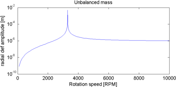
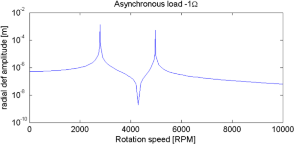
Following example computes frequency response to unbalanced or asynchronous load:

   model=d_rotor('TestShaftDiskMdl'); % Model Initialization

   % Assemble nominal matrices:
   model=fe_caseg('assemble -reset -secdof -matdes 2 1 70',model);
   
   % Campbell diagram and critical speeds:
   fe_rotor('campbell -full -critical',model,linspace(0,20000,30));
   set(gca,'ylim',[0 350]);
 
   % Unbalanced mass or asynchronous load :
   mb=1e-4; db=0.15; % mass, distance to axis
   s=1; f0=1; % s=1, unbalanced load. s<>1, asynchronous load
   om=sort([3296 3200:10:3500 linspace(0,20000,101)]); % RPM

   % RotatingLoad NodeId f0 theta0 exponent : define complex rotating load
   if s==1 % unbalanced mass
    model=fe_rotor(sprintf('rotatingload 2 %.15g -90 2',mb*db),model);
   else % asynchronousload
    model=fe_rotor(sprintf('rotatingload 2 %.15g -90 0',f0),model);
   end
   r1=struct('Omega',om/60*2*pi,'w',s*om/60*2*pi); % Range
   model=stack_set(model,'info','Range',r1);
   R1=fe_rotor('forcedresponse',model); % compute forced response
   iiplot(R1) % plot response
   % Post (radial deformation):  
   Q=max(abs(R1.Y),[],2); figure;semilogy(om,Q);
   xlabel('Rotation speed [RPM]'); ylabel('radial def amplitude [m]')
   if s==1; title('Unbalanced mass')
   else;    title(sprintf('Asynchronous load %.15g\\Omega',s))
   end

Figure 4.10: Top: Campbell diagrams. Bottom: Responses to unbalanced mass and asynchronous load.

Fig 4.10 shows the radial deformation response for an unbalanced load and for an asynchronous load rotating at −Ω speed. The unbalanced load excites the forward modes (3296 RPM) whereas the asynchronous load excites the backward modes (2785 RPM and 4697 RPM). Frequencies match those computed as critical frequencies in the Campbell diagram.

4.3.2 1D models in a rotating (body-fixed) frame

While this representation is not very classical, it corresponds to the nominal choice when doing time integration of a rotor that is not axisymmetric.