PDF Index
| SDT-nlsim
Contents
Functions
PDF Index |
This section aims at presenting the algorithms implemented in the contact module for SDT.
This section aims at presenting how the contact-friction models are be applied to a 3D finite element model using the contact module notations. The main idea to keep in mind is that the relevant contact information is the pressure field transmitted between surfaces.
The first feature to implement is the gap between two solids, as presented in figure 3.1. A slave/master strategy is commonly employed, so that the gap is evaluated by the projection of a contact point of the master surface onto the slave surface.
Practically, the gap between two surfaces is defined as the relative displacement along the contact normal N with a possible offset g0, as
| (3.6) |
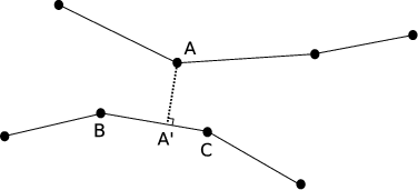
For a 2D application, as illustrated in figure 3.2.1, contact point A is projected as A' on the slave surface, defining the gap as distance AA'. For a displacement u, the displacement of A' is expressed as a combination of the displacements of B and C, which are nodes of the slave surface model.
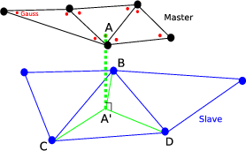
For a 3D application, as illustrated in figure 3.2.1, the computations become more complex in implementation. This case is illustrated in more details as it corresponds to the actual implementation in SDT contact module.
Once master and slave surfaces are identified, the so called contact points must be chosen. They will be the points where contact-friction forces will be actually computed for the mechanical equilibrium. In practice, they are points of the master surface, typically, the surface nodes are chosen, or in our case, the Gauss integration points of the underlying elements (red dots in figure 3.2.1). The interest in choosing Gauss points for contact resides in the fact that an element-wise handling is permitted which allows usual integration rules to be employed and simplifies handling of surfaces for the definition of contact pressures.
The identification of the projected A' of contact point A is referred as the pairing operation, as each contact point of the master surface must be paired to the slave surface depending on its configuration.
In practice, each contact point is first paired to an element of the slave surface, found as being the element in intersection with the outer normal of the contact point. The projected point A' is then expressed in position as a linear combination of the slave element points, B, C and D, which is commonly named mapping. Points B, C and D ∈ NSe the set of nodes of slave element e, they are computed using the shape functions of the slave element. They can be directly exploited, writing
| (3.7) |
where ξk(A′) are the coefficients relating the position of A' in e.
The gap defined by equation (3.6) can consequently be expressed for a contact point mj as
| (3.8) |
In practice, the gap will be expressed at the contact points, but obtained from the mesh deformation u described by the DOF vector q. The practical equation to be exploited is then for a contact point j,
| (3.9) |
where NMe (resp. NSe) are the master element nodes containing (resp. the slave element nodes paired) with contact point j. ξk(A) (resp. ξk(A′)) are the coefficients relating the position of contact point A in the master element (resp. of the projection A′ of contact point A on the slave element). qk is the displacement of node k.
Equation (3.9) is a linear combination of the system DOF, so that it can be summarized using an observation matrix [CNOR]. The gap vector expressed at each contact point is then written
| (3.10) |
noting N the number of system DOF, and Nc the number of contact points.
The generalized force resulting from the gap-pressure relationship, with the gap defined at each Gauss point by equation (3.10), is then defined as
| (3.11) |
where fN is the generalized contact force, p the contact pressure, q a virtual displacement, q the displacement, xj(e) are the integration points of current element e, J(e)(xj) the Jacobian of the shape transformation (surface associated to each integration point) and ωj(e) the weighting associated with the integration rule of element e.
The use of observation matrix [CNOR] is also possible, so that in practice the generalized contact force is expressed as function of the local contact pressure as
| (3.12) |
The computation of the sliding velocity requires the computation of the differential velocities of the slave and master surfaces,
| (3.13) |
where T represents the directions in the friction plane, defined as orthogonal to the contact normal N. T can consequently represent two directions, and the sliding velocity vector be of size 2 Nc. The same developments than for the computation of the gap can be performed, leading to the generation of a tangential displacement observation matrix [CTAN], from which the sliding velocity is
| (3.14) |
and generalized friction forces can be recovered, from the local friction constraint ftj
| (3.15) |
In practice the [CTAN] matrix is expressed sequentially on both local directions of the friction plane,
| (3.16) |
For applications where an externally driven motion exists, the relative displacement of slave and master surfaces becomes a combination of a rigid displacement and a vibration field. In the case where the enforced motion is in the main friction direction, it can be convenient to switch to an Euler description for the external motion. In such formulation, the material is considered to be moving inside a fixed mesh. Additional terms are thus added to the relative displacement observation. The significant benefit is that matching and observation matrices can be generated once.
In practice, a drive speed in the sliding motion direction is added to the relative velocity observation. For rotating devices, one considers a rotating local frame. The rotation effect must then be directly taken into account in the system mechanical equations, which will be referred as an Eulerian formulation. As proposed by Moirot [24], the mesh will remain fixed while the disc material rotates inside. Numerically, the continuous displacement u of the disc can be expressed in the rotating frame as
| (3.17) |
The frame is considered to rotate at a constant velocity Ω, around the ez direction. As the time span possible from the transient simulations provided in chapter ?? is in the order of the tens of milliseconds the effect of the disc slowing down is neglected, so that
| (3.18) |
The velocity of the disc can then be derived from equation (??) considering the total derivative of u, which implies the variations of u as function of its time dependent parameters and the rotation of the base vectors,
| (3.19) |
which can be simplified using (3.18),
| (3.20) |
The sliding velocity is the difference between the disc velocity computed in the rotating frame in equation (3.20) and the velocity of the pad defined in the fixed frame, so that
| (3.21) |
The disc rotation provides a natural sliding direction. It was thus chosen in this work to ignore radial velocities. The projection of equation (3.21) on eθ yields
| (3.22) |
where the product (ez ∧ u ) · eθ from the projection of equation (3.21) on eθ is simplified as the projection of the positions on the radial direction.
In (3.22), the sliding velocity can be decomposed in three contributions from left to right a vibration, convection, and rotation terms can be observed. The first one comes from the fixed mesh vibrations, which are actually computed on the system. The rotation term is constant and only depends on the mesh original topology. The convection term is more difficult to implement as it implies spatial derivations in cylindrical coordinates with a mesh in Cartesian coordinates. This term is thus ignored in [25].
Within an element, displacement u is related to degrees of freedom q through shape functions N
| (3.23) |
the convection term is derived as
| (3.24) |
where xj represents the Cartesian directions.
In the contact implementation used for this work, shape function utilities of SDT are used to generate an observation matrix [CNθ] relating convective contributions of the sliding velocity to the vector of DOF q as in equation (3.24).
In practice, the sliding velocity is thus computed using
| (3.25) |
where the tangent displacement observation matrix [CTAN] has been projected on the tangential direction eθ, and {r} is the radius of each contact point to the rotating frame origin. The names use for generalized strain components are wutt for Ω [CNθ]Nc × 1 {q}N × 1 and wrg for Ω{r}Nc × 1 is included in the vnl(:,:,2).
The effect of the convection term is interesting to interpret, it accounts for the fact that the disc has a static Eulerian deformation due to friction. The disc slows down entering the pad area and accelerates when existing. The effect is obviously a linear function of the friction coefficient.
The disc rotation also has an effect on the expression of the acceleration for the formulation of the mechanical equilibrium. The acceleration of the disc is defined as
| (3.26) |
which is obtained by deriving equation (3.20),
| (3.27) |
where r is the projection vector on the tangent plane {er ;eθ ;0}.
Equation (3.27) presents several additional terms to the displacement acceleration ∂2 u/∂ t2. From left to right, a gyroscopic damping associated to the first order time derivatives of u (2Ω factor), a gyroscopic stiffness associated to the θ only derivatives of u (Ω2 factor) and a volume centrifugal load are identified.
The mechanical equilibrium equation should then be altered to stand for all rotational effects in the disc. In practice however, the disc rotation velocities targeted are rather small - a few rad/s - so that all gyroscopic and centrifugal terms are neglected, for squeal applications, thus leading to
| (3.28) |
Adjusting rotation related terms in the equilibrium equation is a perspective for future work.
When characterizing a non-linear system in the frequency domain, the most common approach is to consider the system linearized around a deformation state and compute the modes of the linearized system. The linearized model is then called tangent to the said deformation state. This strategy is of course limited, as linearizing in the vicinity of deformation states can only be relevant for very small deformations from the targeted working point.
The expression of the system linearization strongly depends on the chosen contact formulation. For Lagrangian formulations, the definition of the tangent state only depends on the surface effectively in contact, as a contact point is either open (no contact) or closed (in contact). The open case generates no contact stiffness, while the closed case generates an exact continuity constraint for the normal displacement at the interface.
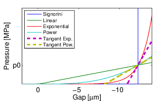
Constitutive contact formulations are defined as function of the gap, such that a tangent state can be derived for each contact point by deriving the gap/pressure relation as illustrated in figure 3.8. It should be noted that the contact stiffness differs at each contact point and depends on the local gap.
At a given contact point i the contact stiffness kci is defined by the derivative of the pressure gap relationship,
| (3.29) |
where pi is the pressure at contact point i, J(xi) the corresponding surface, and ωi the Gauss weighting coefficient. Using the gap observation equation (3.10) and the force restitution of equation (3.12), the tangent contact stiffness matrix Knlc (q) is recovered,
| (3.30) |
Knlc is therefore symmetric positive definite and can be used for real and complex modes.
The effect on the system itself is a perceived stiffness variation occurring at each point of the contacting interfaces. The distribution of contact stiffness can then show large variations over the surface.
The definition of a tangent friction state is more difficult, as it couples normal and tangential directions, it is typically non-symmetric - thus being a common source of instability.
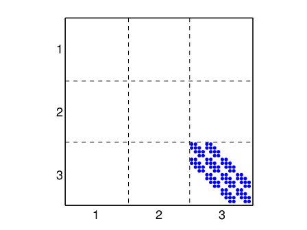
The nature of friction as written in equation (3.2) shows that a variation of contact force has a direct effect on friction force, while a variation of the friction force may occur without effect on the contact force. This non symmetric notion is illustrated in figure 3.9 where stiffness coupling matrix topologies are illustrated for a basic case.
In the case of a sliding state, the friction force is explicitly defined and only depends on the contact force at the same point. The tangent friction is then the tangent contact (3.29) scaled by the friction coefficient µ, linking the normal and tangent displacements for complex modes. For real mode computation, since the tangent displacement is free for a fixed contact state, no stiffness is added. The tangent friction coupling stiffness Knlfslide for sliding states is defined as
| (3.31) |
The formulation of tangent friction matrices of equation (3.31) is very classical, and is commonly employed under the small sliding perturbations formulation. This was used by Moirot [24], Lorang [25] for brake squeal applications, or by Vola et al. [26] to study rubber/glass instabilities in sliding steady states.
Sticking friction state is very different in application. The basic Lagrangian approach will consider an exact continuity constraint of the tangential displacement at the interface, thus making it a bilateral constraint. Taking such pattern into account is critical for the complex modes as a physical resistance to the tangential displacement occurs. For sliding to happen, the friction force must increase up to the sliding threshold, this friction force variation must then be reproduced.
A functional approach can be used, which relaxes the Lagrange constraint. The friction force is however unknown inside the Coulomb cone, and further studies are necessary to characterize the stiffness coupling levels and the system sensitivity. Experiments are suggested by Bureau et al. [27] for non metallic materials. Ultrasonic measurements as done by Biwa et al. can also be a possibility [28]. In particular Biwa proposed a link between the sticking state stiffness and the interface material properties.
The strategy chosen here is to consider the Coulomb cone limit, characterized by the contact force level, illustrated in figure 3.2. A proportional relationship linking the tangent friction stiffness level and contact levels is set, using parameter κ. The stiffness behavior will thus be close to microslip patterns, occurring for low vibration levels. Obviously κ, which has to be somehow identified, will verify
| (3.32) |
The tangent friction coupling stiffness Knlfstick for sticking states is then defined for both real and complex mode computation as
| (3.33) |
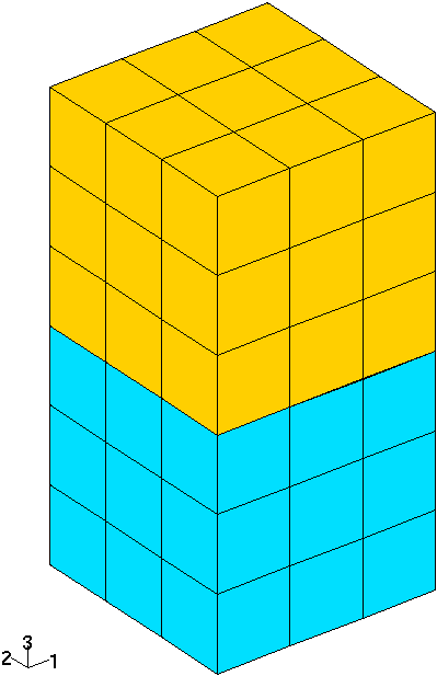
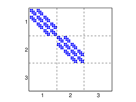
To illustrate the effect of the different tangent contact-friction matrices presented here, an example based on a very simple problem is presented. The basic model given in figure 3.9 features two cubes in vertical contact. For illustration purposes, the degrees of freedom are segregated by their direction, 1 and 2 define the horizontal directions while 3 is the vertical normal direction, in which contact is defined.
Figure 3.9 presents the topologies of the tangent contact-friction matrices expressed on the master surface DOF. The tangent contact matrix (3.30) couples the normal directions, here the third one, as shown in figure 3.9. The matrix is symmetric positive definite and used for real or complex mode computation.
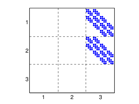
The tangent friction matrix (3.33) for sticking states is plotted in figure 3.9. It couples directions 1 and 2 independently, is symmetric positive definite and is used in real and complex modes computation.
For sliding states, the tangent friction matrix (3.31) is shown in figure 3.9. The un-symmetric coupling is clearly observed as direction 3 is coupled to both directions 1 and 2. A deformation along 3 has an effect on directions 1 and 2 but not the other way around.
Partial support of large displacement surface contact problems is being implemented for point (node or Gauss) to surface contact (look for the ScLd tag) . The generalized strain stored in unl is
xp,yp,zp, g,r,s,ielt,wjdet,n3x,n3y,n3z
corresponding to 3 strains and 8 internal states. The 3 strains are the current position of the contact point obtained as xp=xp0+uxp. The gap is the first internal state and is counted as positive if the point is outside the surface (there actually is a gap rather than penetration). r,s give the position within current the triangular element of C index ielt. wjdet is the weight associated with the point needed to apply a load and n3i are the components of the normal vector specifying the direction of the normal load.
The unl0=unl(:,:,2) stores xp0,wjdet,n3x,n3y,n3z which do not change. g of the previous time step which can be used for laws that use time derivatives of g. r,s,ielt of the previous search which is used to speed search of the next point.
A residual call performs the following steps
This unsupported development is found in oscar_panto BBeam.
cont_laws.tex