PDF Index
| SDT-nlsim
Contents
Functions
PDF Index |
This section presents the two most classical ways of modeling contact friction interactions between structures. First physical models are described, then numerical implementation for finite element models is presented. Finally tangent contact friction derivation strategies are presented for modal computations.
The simplest contact representation - at least in formalism - is commonly known as the Signorini-Coulomb law to relate contact and friction. The definition of contact between to solids requires the notion of gap giving the distance between the solids considered, and taken as positive if non contact occurs. The notion of contact normal naturally follows as giving the way of measuring the gap. As presented in figure 3.1, the gap is measured as the shortest distance between two solids thus along the normal between both solids. It is function of the deformation u of each solid.
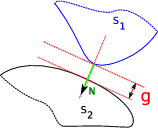
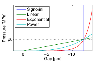
Figure 3.1: Contact normal (N) and gap (g) definition for two solids, and the Signorini contact-pressure law.
In case of contact, a reaction force exists between both systems to avoid interpenetration. As contact between three dimensional solids is a surface, the notion of contact pressure is preferred here, and will be denoted p. It is of course directed by the contact normal. The Signorini conditions thus states for each point in contact
| (3.1) |
which sets exclusion between the gap values and contact pressure values. Two states are then possible, opened contact with a strictly positive gap and closed contact with a null gap and a strictly positive contact pressure. The law is plotted in figure 3.1. It is worth noting that Signorini contact is a mathematical idealization that is incompatible with the physics of surface irregularity at smaller scales.
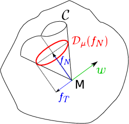
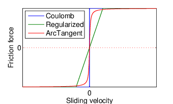
The ideal Coulomb friction, as originally presented considers a so-called static friction model. The formulation distinguishes sticking and sliding states, depending on the existence of movement between the bodies in contact. If the solids in closed contact do not slide, a reaction force - the friction force - exists between both. This force is in the tangent plane defined as orthogonal to the contact normal N, and is determined by the equilibrium of the whole system. In the case of sliding, the friction force is opposed to the sliding velocity w, and only proportional to the normal load (or contact pressure) through the introduction of a friction coefficient µ.
Coulomb friction can be expressed as
| (3.2) |
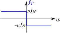
where fN is the contact force, fT the friction force, µ the friction coefficient, and w the sliding velocity. The law is plotted in figure 3.2 which represents the friction force as function of the sliding velocity. For non-sliding states, the friction force is not defined by the law, as only an inequality is set.
The inequality concept is classically represented by the Coulomb cone shown in figure 3.2. For a given contact force at point M, the reaction force is said inside the coulomb cone Cµ, and more precisely in the cone section Dµ, determined by the tangent plane direction and the contact force amplitude.
The Signorini-Coulomb laws given by equations (3.1) and (3.2) raise numerical and analytical issues, since contact and friction forces are not defined for each point of their parameter. Indeed, for zero sliding velocity and zero gap, the forces are unknown and must be determined by other means.
To solve such problem a Lagrangian formulation has to be used, where the contact-friction forces are considered unknown and kept in the system to solve. The system size thus increases as function of the number of contact points, and features inequalities.
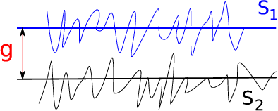
In addition to the numerical difficulties due to the Signorini-Coulomb formalism, the idealization represented may not always be satisfying. The reality of surfaces is indeed roughness describing the irregularities coming from the asperities of both surfaces [23]. This is conceptualized in figure 3.3.
Due to the very small scales of these asperities - around the micrometer - they are obviously not modeled in details. The roughness measures in particular commonly realize statistics on the whole surface, yielding a few parameters describing the surface state. Of course simulation of mechanical components consider nominal surfaces, with no asperities, as represented in figure 3.3.
In the world of asperities averaged by a nominal surface, interpenetration is possible at the macroscopic level, as function of the pressure applied on both surfaces. Indeed, the compression of asperities then increases allowing a greater contact pressure. From macroscopic tests, it is thus possible to obtain a law relating gap to contact pressure.
Possible functional representations of the pressure/gap relation are linear, power series or exponential laws, illustrated in figure 3.4.
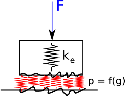
In practice, the contact pressure is applied to a deformable body. Assuming a certain height for this body, its stiffness ke can be defined. The measurable displacement is related to pressure by
| (3.3) |
which is illustrated in figure 3.5.
Extreme regimes can easily be seen in equation (3.3). For a very thin body, the stiffness ke is very high and the deformation will be mostly due to the deformation of asperities. In such case, a pressure/gap relation should be used.
For many more configurations, the gap induced by realistic pressures will be small compared to deformations in the body. This regime is the reason for the widespread use of Signorini conditions. Since the real penetration is small, it cannot be measured accurately against body deformation and assuming it to be zero thus makes more sense. Furthermore, using it would cause major numerical difficulties since the accuracy on gap increments would need to be much higher than the accuracy desired for global motion.
Functional representations of contact pressures are also called penalization when the function is seen as a numerical tool rather than the result of an homogenization due to scale separation. In such case, gaps obtained in the simulation are (incorrectly) seen as numerical approximations. A relaxation of the Lagrange constraints is thus performed, authorizing interpenetration whose trade-off is the addition of a force linked to the violation of the constraint. The best interpretation is obtained energetically, where the relaxed constraint violation is generates a highly energetic term. Consequently, the mechanical solution will only show limited violations of the constraint.
It is noted here that the zero gap value that would be used in a Signorini model does not normally correspond to zero pressure, the contact of the mean smooth surfaces considered in this case corresponds to a state where some asperities are already into contact.
Using such laws, contact forces can be condensed on the displacement, making mechanical resolution much simpler. Contact law parameters must however be identified experimentally which may be difficult, whereas Signorini requires numerical adjustments. Contact mechanism is well assessed, and both Lagrangian and functional formulations have their adepts.
Practically the chosen contact model must be capable of properly transmitting pressure fields through the interface. To behave physically, the contact model should generate interpenetration at the expected scale and provide a coupling stiffer than the normal compression of the structure observed from the interface. If these aspects are respected, the structure will be able to see proper pressure fields at its interface.
It can be noted that non-linear functional representations, such as the exponential law (section 3.3) provide tangent stiffness fields varying with the gap, over the surface thus reflecting in the modal domain the effect of loading on the surface. Other laws, like the linear functional law or exact Signorini will provide the same tangent state whatever the contact pressure distribution if the contact surface remains identical. In such case, non-linear simulations are necessary to evaluate the effect of load variation over the surface.
One should also note that in finite element simulations, the appropriate model will depend on element size with, functional representations being more appropriate for small elements. More generally, computation with compatible meshes should be preferred. Contact simulation with non conforming interfaces can generate peculiarities that should require specific care, at least verification from the user.
Friction behavior is more complex, and the Coulomb law, as simple as it is, does not satisfy the needs of everybody.
On the first hand, regularization methods can be employed to relax the Coulomb law for zero sliding velocities. The idea is then to penalize low sliding velocities through the introduction of a slope at the origin, introducing a parameter kt, so that
| (3.4) |
as shown in figure 3.6.
The basic regularization given by equation (3.4) is not perfect. First the threshold level will depend on the contact pressure
as its regularity is low, indeed, it is not differentiable at its transitions. An arctangent law can be used to alleviate the problem,
| (3.5) |
Two main drawbacks exist with such regularization. First, parameter kt does not have a clear physical meaning, so that its value is difficult to determine. In particular, when dealing with distributed contact on large surfaces, the contact pressure will be shown to have major variations over the surface. The use of a constant kt may thus be a problem.
Second, the regularized contact laws loose their static capability. In (3.4), a case with no sliding velocity implies no friction force. This is not compatible with stuck states when friction force is needed to maintain the sliding velocity to zero. Only stick-slip transition can then be approached for a globally sliding configuration.