8.2 SDT Tabs
This section presents the GUI of SDT, organized as tabs in the sdtroot figure.
-
The application tools breakdown is provided in an exploration tree placed at the figure left. The buttons allow opening the corresponding interface tabs.
- The tab area displays interactive tables that allows parameter editing and procedure execution. User interaction is associated with tabs implemented in the GUI,
-
Project tab to handle the working environment, section section 8.2.1.
- FEMLink tab to handle model imports, section section 8.2.2.
- Mode tab to handle modal computations, section section 8.2.3.
- TestBas tab to superpose two meshes, section section 8.2.4.
- Ident tab SDT identification tuning, section section 8.2.6.
- StabD tab for stabilization diagrams, section section 8.2.5.
- MAC tab to handle MAC analysis, section section 8.2.7.
- OsDic tab for sdtroot OsDic editing, section section 8.1.3.
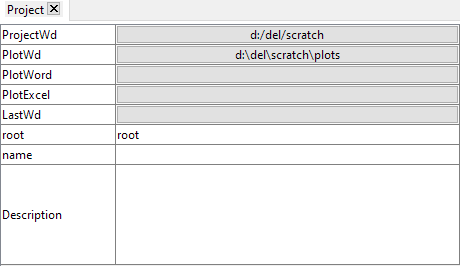
8.2.1 Project
The Project tab allows handling the working environment.
This is a 2 column table allowing the definition of the following fields,
-
ProjectWd A button defining the working directory used for the project. This is where models and curves will be saved. Clicking on the button will open a dialog for interactive definition.
- PlotWd A button defining the directory where image captures will be saved. If not specified the default will be ProjectWd/plots. Clicking on the button will open a dialog for interactive definition.
- PlotWord A button defining an existing Word report to which captured images can be inserted. Clicking on the button will open a dialog for interactive definition.
- PlotExcel This is not currently used, but could allow the specification of a different file for table export.
- LastWd The last chosen directory, used as a starting point for the next directory selection dialogs.
- root A short name that will be used to identify saved files in the project working directory, every saved file will start with this root.
- name A longer name version that is used for human description of the project name.
- Description An optional text that can provide further details on the current project.
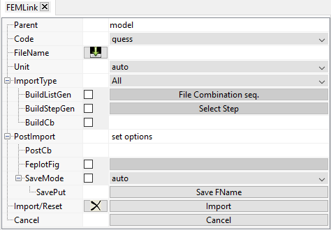
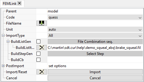
8.2.2 FEMLink
The FEMLink tab allows handling model import from external codes.
This is a three column table allowing interactive definition of the fields described below. The second column allows activating specific options.
-
Parent string name used to identify the model in further post-processing operations.
- Code allows selecting the code from which files will be imported. If code is unknown femlink will try guessing it from the file extension. This is a popup button providing a specified list of options. This is set by default to unknown.
- FileName Provides the base file for import. This file will be imported first and constitute the base model for the output. The second column button allows an interactive file selection through a dialog. The third column is an editable text cell.
- Unit allows defining a unit system with the model, that can be used for post treatments where output units are required. Some codes do not use it so that an external definition is needed. This is set by default to auto.
- ImportType Provides model building options based on complementary files
-
All imports model, results, ...
- Model just imports the model, material properties, boundary conditions, ...
- Result import result.
- UPCOM SE import element matrices in a type 3 superelement handled with upcom.
-
BuildListGen allows generating a file list sequentially built, by successive file selection. These files then appear under the BuildListGen button and can be removed from the list by clicking on
 . This is illustrated in figure 8.4. This option conditions the activation of BuildStepGen and BuildCb below.
- BuildStepGen : Should be updated with a capture of the window for step selection. Allows defining model Case resolution for a specific results step. By default femlink imports all data in the model. To recover specific boundary conditions relative to a specific computation step (if defined in the input and supported by the femlink function), one can either provide the step number or ask for last to let femlink find the last step defined in the model load case. The third column button allows selecting a step in an interactive way. By default, this option not is activated.
- BuildCb Allows defining further Build commands that may depend on the Original Code selected. The second column activates the option. The third column button provides a series of comma separated calls that will be applied to the model generated by femlink through the FEMLink function defined by the Code.
- PostImport is used to define steps performed after the base import.
-
PostCb callback performed after import (for custom applications using FEMLink).
- FeplotFig Allows direct model loading into a feplot figure for visualization. The second column button activates the option. The third column button allows interactive selection a feplot figure, like for the Project tab. By default, this option is not activated.
- Save allows defining model saving strategy once imported. The second column button activates the option. The third column button allows defining a saving mode. This is a popup button proposing either :
-
auto that will perform an automatic saving of the model based on the Mesh File name with a _import.mat extension
- Link to Project that will use the Project tab data to generate a file name. In this case the saving file name will be Project.root _ date _ Mesh File name _ import.mat
- Custom fname allows defining a user specific name in the second line button. The Save FName button can then be clicked on to provide a file name that will be used as verbatim.
By default the save option is activated and set to Link to Project.
- Import/Reset Import executes the import procedure. The cross resets the tab to its original state.
| Figure 8.4: The FEMLink tab, filled with input files |
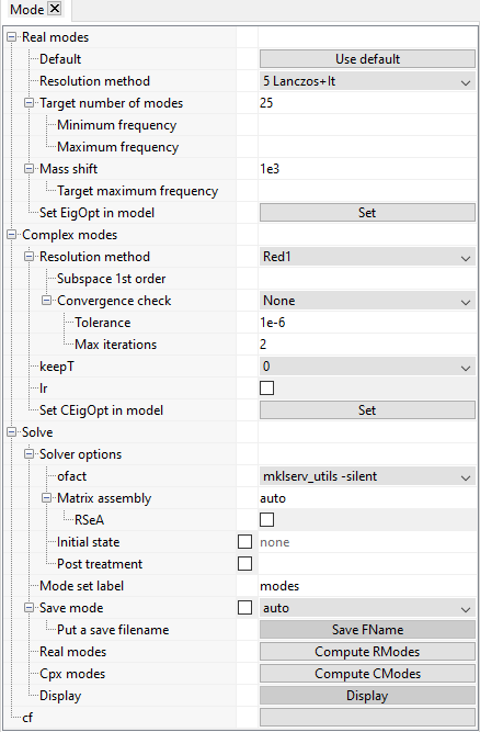
8.2.3 Mode
The Mode tab allows handling modal computations.
This is a three column tree-table allowing various choices to perform a wide range of modal computations, parametered by the fields below,
-
Real modes This section and the associated sub-tree provides options on the computation of real modes
-
Default Resets parameters of the real mode sub-tree to default values
- Resolution method The real mode solver (resolution method) choice (also used for reduced complex mode computations). Choices are packaged in a popup cell :
-
Lanczos+It : set by default and recommended
- Lanczos : same as the previous without convergence check and correction, be used once parameters are calibrated
- IRA/Sorensen : quicker but less robust
- Target number of modes To provide a number of modes to compute, set to 25 by default.
-
Minimum frequency To provide a minimum frequency of interest (not packaged yet).
- Maximum frequency To provide a maximum frequency of interest.
- Mass shift To provide a mass shift used for the factorization. This is set to 1e3 by default.
-
Target maximum frequency To provide clues on the expected bandwidth (will influence the mass shift).
- Set EigOpt in model
- Complex modes This section and the associated sub-tree provides options on the computation of complex modes
-
Resolution method The complex mode solver (resolution method) choice. Choices are packaged in a popup cell either :
-
Red1 : complex modes on the real mode subspace (default)
- Red2 : complex modes on the real mode subspace enhanced with the imaginary part of the stiffness
- Full : direct without reduction
-
Subspace 1st order The choice of the matrix types to be used for the subspace enhancement. The visc option is only available with SDT-visco licenses.
- Convergence check Not packaged yet.
- keepT
- lr
- Set CEigOpt in model
- Solve This section and the associated sub-tree provides options on the solver to use and potential post treatment or saving strategies.
-
Solver options
-
ofact The choice of the matrix factorization solver, set by default to mklserv_utils -silent. This is recommended for very large models.
- Matrix assembly A text cell providing the matrix types to be assembled for the computation. This is either the keyword auto to let the solver decide the assembly strategy, or a series of matrix types (see sdtweb mattype) to be assembled. By default this is set to auto, corresponding to 2 1 for real modes and 2 3 1 4 for complex modes.
- Initial state This is activated by the second column. The third column provides a callback to initialize the system state. (not packaged yet).
- Post treatment Allows performing a callback after mode computation. The second column activates the option. The third column is a text cell providing a callback to perform. Not packaged yet.
- Mode set label A curve name used to store the deformation curve in the model stack. This is a text cell, set by default to modes.
- Save mode allows automatic curve saving once imported. The second column button activates the option. The third column button allows defining a saving mode. This is a popup button proposing either :
-
auto that will perform an automatic saving of the curve based on the base model name with a _def.mat extension.
- Link to Project that will use the Project tab data to generate a file name. In this case the saving file name will be Project.root _ date _ model name _ Mode set label _ def.mat
- Custom fname allows defining a user specific name in the second line button.
-
Put a save filename The Save FName button can then be clicked on to provide a file name that will be used as verbatim.
- Real modes Executes the real mode computation
- Cpx modes Executes the complex mode computation
- Display Displays the model stack entry named after Mode set label.
- cf A button allowing an interactive definition of the feplot figure that will hold the working model. Clicking on the button opens a dialog interface proposing the selection of an existing feplot figure or to open a new one. By default, this is set to the one specified in the Project tab.
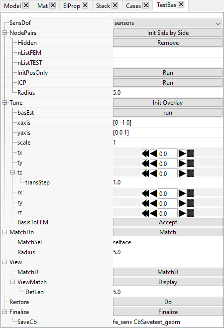
8.2.4 TestBas : position test versus FEM
The TestBas tab is used to superpose two meshes. For examples see section 3.1.
This is a tree-table used for mesh superposition. The base mesh is called FEM and the mesh to be placed is called TEST even when you are superposing different things (TEST/TEST, FEM,FEM, ...). The NodePair section uses a strategy providing corresponding points, while the Tune section allows manual tuning of the relative position.
-
SensDof selects the second mesh (stored in as a SensDof case entry in the first mesh) to be superposed on the first one.
- NodePairs is used to initialize the FemTest dock in side by side mode. In this mode, the left tile shows the feplot promodel, the center tile shows the reference mesh and the right tile the SensDof mesh.
The first step in this mode is to provide two list of paired nodes for the two meshes. To select the nodes, select a feplot figure and press the space bar: clicking on the mesh will select nodes and add them to the list. Doing so in the two feplot figures provides two sets on paired nodes that can be used superpose with this information only (InitPosOnly) or with the help of an automatic algorithm after the initial positioning (ICP : Iterative Closest Points).
-
Hidden To ease selecting only visible nodes on each mesh, this button removes hidden elements from the camera point on view. (Useful when selecting the paired node lists)
- nListFEM list of nodes selected in the main mesh feplot in center tile.
- nListTEST list of nodes in SensDOF mesh (right tile).
- InitPosOnly superpose the two meshes by minimization the Euclidean distance between the previously filled lists of paired nodes. This is helpful in presence of geometries with symmetries for which the ICP algorithm cannot converge (plate or cylinder for instance).
- ICP, using paired node lists, performs first the InitPosOnly action and then starts the optimization with the algorithm ICP which seeks to minimize the point-to-plane distance between each automatically paired nodes (closest nodes in the range of Radius).
- Radius search radius for node pairing (this is the same value as the Radius in MatchDo)
- Tune opens the FemTest dock inTune mode. The left shows the feplot promodel while the right feplot overlays the reference mesh (in blue) and the test mesh in its current position (in red)
-
basEst : starting guess : if no InitPosOnly has been performed, the two meshes are automatically superposed using the gravity center and the three main directions of the point clouds formed by each node mesh. This is helpful to be closer to the good superposition before beginning to tune manually
- xaxis This is an informative display which gives the orientation of the x-axis test coordinate system in the base model. This is updated when rotating the second mesh
- yaxis orientation of test y-axis in FEM coordinates.
- scale scale applied between the two coordinate systems (for FEM in mm and test in meters use 0.001).
- tx Translation of test in the x-direction. The single arrows correspond to a low displacement step and the double arrow to a higher displacement step
- ty Translation of test in the y-direction
- tz Translation of test in the z-direction
-
transStep This is the translation step used by the single arrow.
- rx Rotation of the second mesh around the x-axis. This rotation does not increase the angle which is always zero, but updates the orientation of the xaxis and the yaxis. The text is used for using input of large changes 90 (degrees) for example.
- ry Rotation of the second mesh around the y-axis
- rz Rotation of the second mesh around the z-axis
- BasisToFEM Modify the SensDof mesh by applying the transformation. The node coordinates are modified and all Tune fields set to identity.
- MatchDo Match is automatically performed after ICPPosOnly, ICP and BasisToFEM. This button can be used to redo the match with new options below.
-
MatchSel Selection on the FEM before performing the Match. selface is classically used to force the match on the surface of the model instead of in the volume.
- Radius Search radius for node pairing (this is the same value as the Radius in NodePairs)
- View List of different views to evaluate the quality of the superposition
-
MatchD displays the table showing the gap between each node of the second mesh and the matched surface. It also shows this information as a colormap on the test.
- ViewMatch Displays the test mesh over the FEM with the options listed below
-
DefLen Length of arrows if displayed
- Restore uses the .bas0 field to reset all the modifications since the last BasisToFem (performed after clicking on InitPosOnly, ICP and BasisToFEM) and put the second mesh at this previous location.
- Finalize Performs the SensMatch (i.e. the observation of the first mesh at sensors)
-
SaveCb Callback executed with the Finalize action
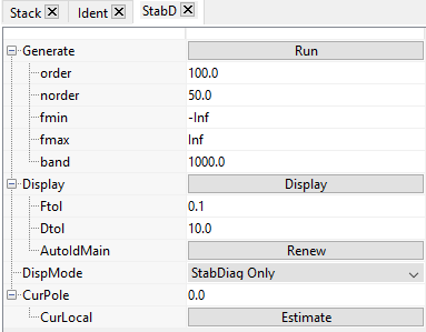
8.2.5 StabD : stabilization diagram
The StabD tab is used create a stabilization diagram with the algorithm LSCF and provide tools to extract poles from it.
This is tab is used for LSCF handling (see section 2.3.2).
- Generate click on button to generate stabilization diagram.
-
order : Maximum order of the model. The order of the model equals the number of poles used to fit the measured data. It is often necessary to select an order significantly higher than the expected number of physical poles in the band because the identification results in many numerical poles which compensate out-of-band modes and noise. Selecting at least ten times the number of expected poles often gives good results according to our experiment.
- norder : Minimum order to start the stabilization diagram (low model orders often show very few stabilized poles)
- fmin : Minimum frequency defining the beginning of the band of interest
- fmax : Maximum frequency defining the end of the band of interest
- band : Sequential iteration can be performed by band of the specified frequency width. The interest is that in presence of many modes, it is more efficient to perform several identifications by band rather than increasing the model order.
- Display : display result
-
Ftol : tolerance for frequency convergence
- Dtol : tolerance for damping convergence
- AutomIdMain : fill IdMain set of poles from current data.
- DispMode
- CurPole : info based on click.
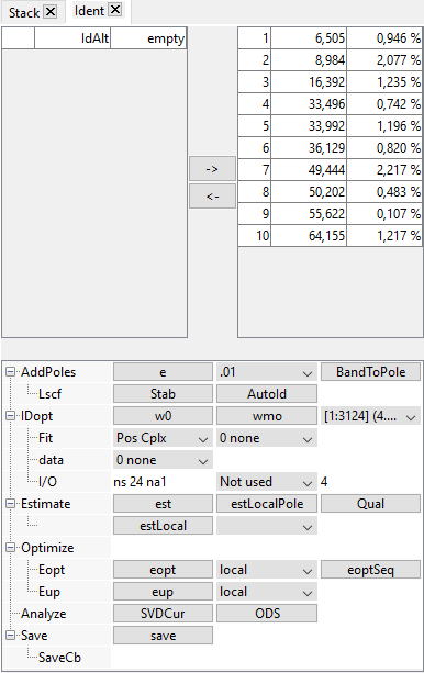
8.2.6 Ident : pole tuning
The TabIdent tab is
The upper part is a list of alternate poles on the left and retained poles on the right. The arrows let you move poles and associated shapes from one list to the other.
The lower part as the main sections
-
AddPoles see section 2.3
-
Lscf LSCF algorithm see section 2.3.2
- IDopt section 2.4
- Estimate section 2.5
- Optimize section 2.6
- Analyze section 2.9
- Save
-
SaveCb allows customization of saving strategy
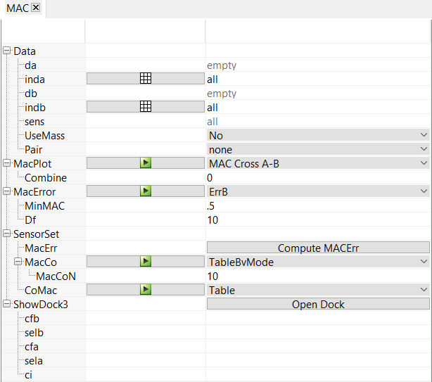
8.2.7 MAC : Modal Assurance Criterion display
The MAC tab allows handling display of variants of Modal Assurance Criterion.
This is a three column tree-table allowing various choices to perform a wide range Modal Assurance Criterion variants, parametrized by the fields below
-
Data Options to properly define input data
-
da provides indications on the number of sensors and the number of modes of
- inda
- db
- indb
- sens
- UseMass
- Pair
- MacPlot
- MacError
- SensorSet
- ShowDock3
©1991-2025 by SDTools