
 PDF Index
| SDT-base
Contents
Functions
PDF Index |
Topology correlation is the phase where one correlates test and model geometrical and sensor/shaker configurations. Most of this effort is handled by fe_sens with some use of femesh. The graphical interface is the CoTopo dock shown below.
As described in the following sections the three important phases of topology correlation are
Starting with SDT 6.0, FEM sensors (see section 4.7) can be associated with wire frame model, the strategy where the two models where merged is thus obsolete.
Two types of data are needed to properly associate a test wire frame model to a FEM :
One then declares the wire frame (with sensors) as SensDof case entry as done below (see also the gartte demo). The objective of this declaration is to allow observation of the FEM response at sensors (see sensor Sens).
 [model,TEST]=demosdt('DemoGartDataCoTopo'); % load FEM and TEST wireframe
 % Store Test as SensDof (linked test wireframe) in the FEM
 model=fe_case(model,'sensdof','sensors',TEST);
 cf=feplot(2); cf.mdl=model; % Display the model in feplot
 % Display the superposition of the test wireframe over the FEM
 fecom(cf,'ShowFiCoTopo');
 % Open the CoTopo Dock from cf, already containing needed data
 fecom(cf,'dockCoTopo');
Section 4.7 gives many more details the sensor GUI : the available sensors (sensor trans, sensor triax, laser, ...). Section 4.7.1 discusses topology correlation variants in more details.
If the data come from files, it can be more convenient to load them directly from the GUI.
Here is a tutorial for interactive data loading in DockCoTopo with the TestBas tab.
You will need the garteur example files, which can be found in SDTPath/sdtdemos/gart*.m. If these files are not present, click on the first step on the following tutorial in the HTML version of the documentation or download the patch at the address https://www.sdtools.com/contrib/garteur.zip and unzip the content in the folder SDTPath/sdtdemos.
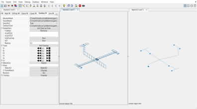
 Execute the command fecom('dockCoTopo') to open an empty dock. You can also click on the button CoTopo on the tree in SDT Root.
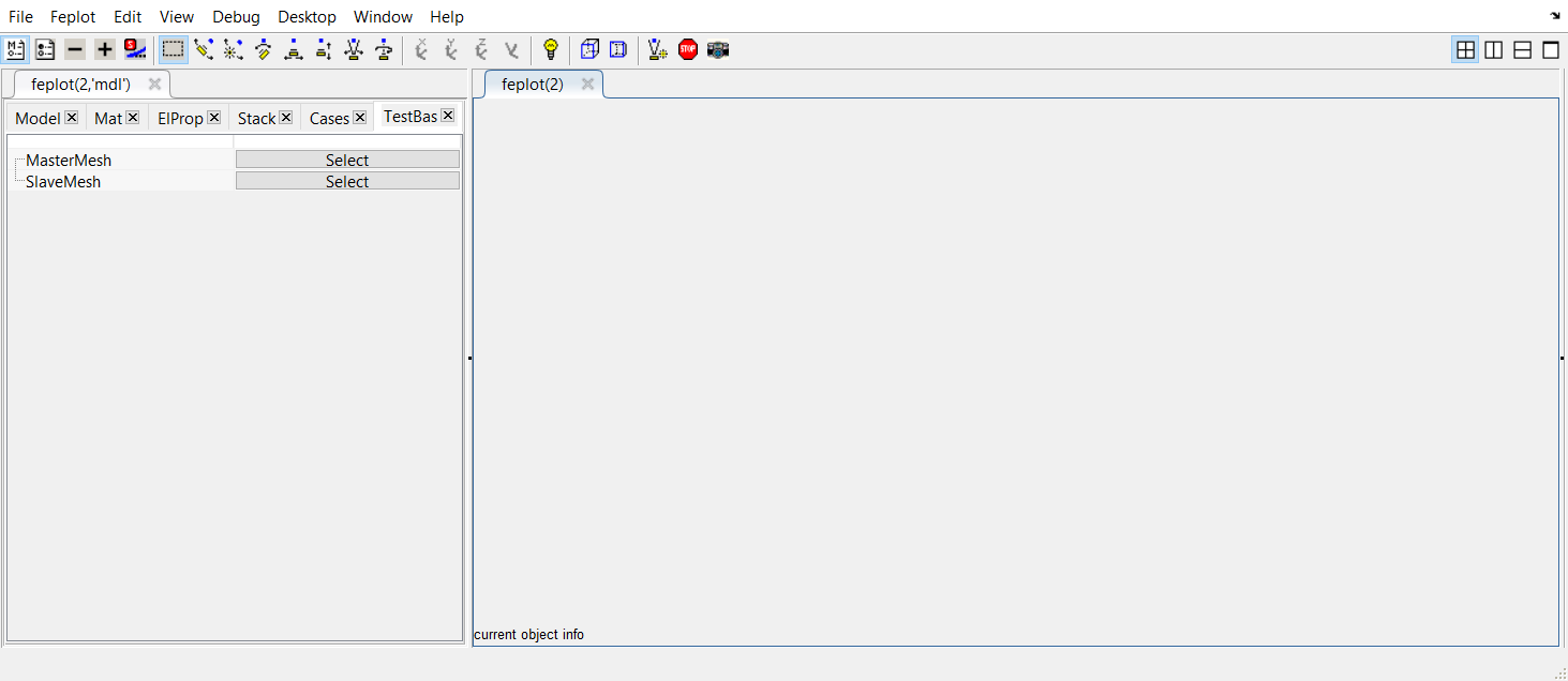
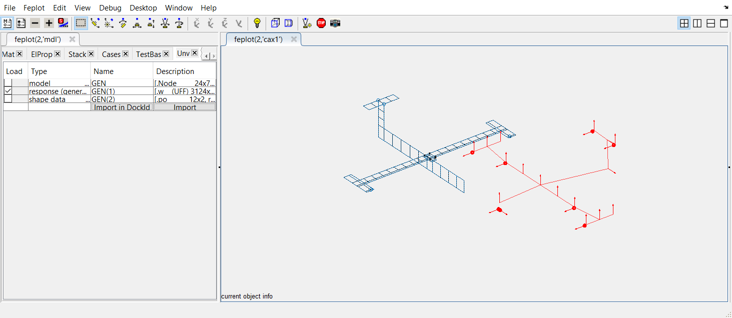
Click on Select associated to MasterMesh. This will open the import model window. Select the file to load : for this tutorial, the file is located at SDTPath/sdtdemos/gart_mdl.inp. Data is loaded and displayed in the feplot figure.
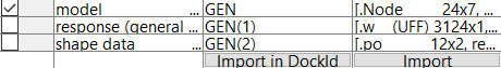
Do the same for the SlaveMesh. The test mesh file is located at SDTPath/sdtdemos/gartid.unv. Data is loaded and displayed in the feplot figure. Once selected, the Unv tab is displayed in the feplot('mdl') figure : it shows the content of what is inside the Unv file.Check the box corresponding to model and click on Import.
The test wireframe is loaded and displayed in the feplot figure in red.
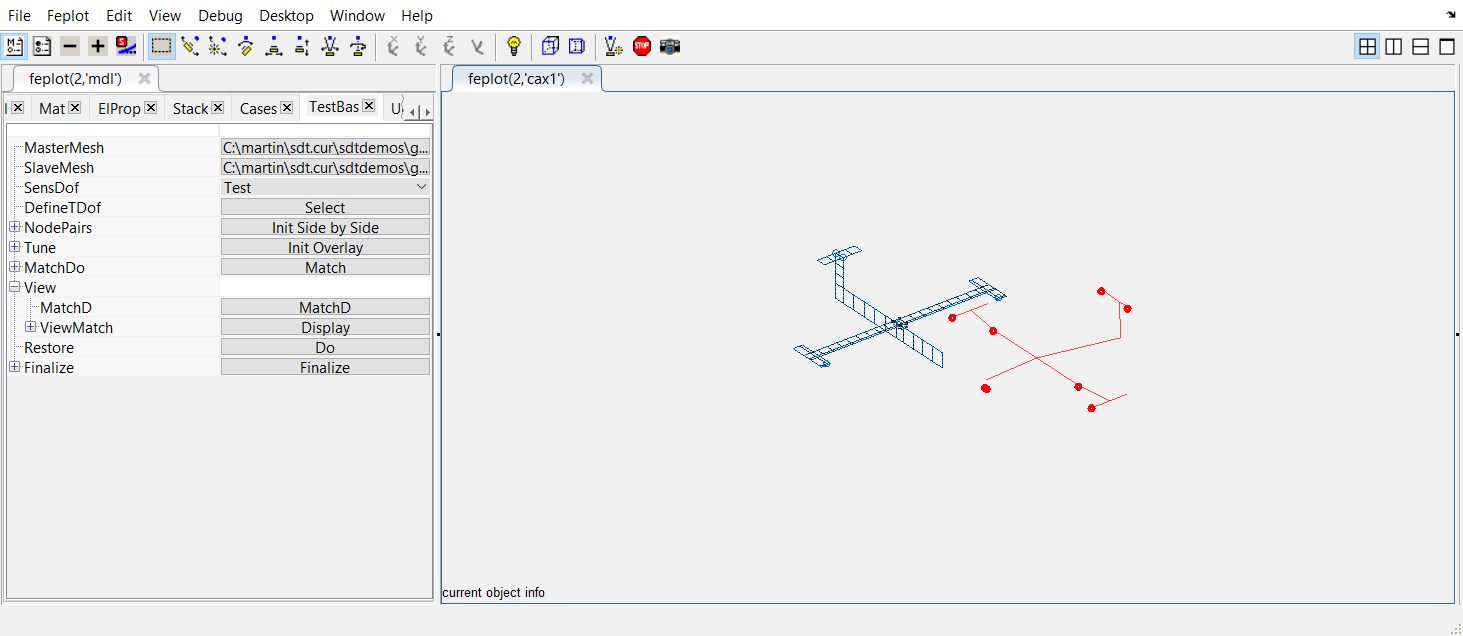
Depending on the loaded data for the the SlaveMesh, it contains already or not the sensor definitions : they are shown as red arrows. It is not the case here.
To retrieve sensors definition from a Unv file, the measured data need to be loaded.Click on Select associated to DefineTDof. Select again the Unv file and in the Unv tab, check this time the box corresponding to response and click on Import.
The arrows are then built depending on the measured channels (+X,+Y,+Z,-X,-Y,-Z directions associated to each nodes in the geometry), and displayed.
The system coordinate is not the same between the test wireframe and the FEM : the test geometry needs to be moved and superposed to the FEM (this tutorial continues in the following subsection).
In many practical applications, the coordinate systems for test and FEM differ. fe_sens supports the use of a local coordinate system for test nodes with the basis command.
Interactive test mesh placement is available in the SDT GUI, using command fe_sensGuiTestBas.
% Loading the interactive test mesh placement GUI
 cf=demosdt('demo garttebasis closeall'); % Load the demo data
 cf.CStack{'sensors'} % contains a SensDof entry with sensors and wireframe
 fecom(cf,'setTestBas'); % Open interactive tab in feplot properties
Operations permitted through the GUI implementation are available in script commands. The modus operandi considers a three steps process.
In peculiar cases, the FEM and TEST mesh axes differ, and a correction in rotation in the Phase 2 may be easier to use. An additional rotation to apply in the TEST mesh basis can be obtained by fulfilling the field rotation in Phase 2. The rotations are applied after other modifications so that the user can directly interpret the current feplot display. The rotation field corresponds to a basis rotate call. The command string corresponding to a rotation of 10 degrees along axis y is then 'ry=10;'. Several rotations can be combined: 'ry=10; rx=-5;' will thus first perform a rotation along y of 10 degrees and a rotation along x of -5 degrees. These combinations are left to the user's choice since rotation operations are not symmetric (e.g. 'rz=5;rx=10;' is a different call from 'rx=10;rz=5;').
The following example demonstrates the 3 phases in a script.
 cf=demosdt('demo garttebasis'); % Load the demo data
 cf.CStack{'sensors'} % contains a SensDof entry with sensors and wireframe

 % Phase 1: initial adjustments done once
  % if the sensors are well distributed over the whole structure
  fe_sens('basis estimate',cf,'sensors');

 % Phase 1: initial adjustments done once, when node pairs are given
  % if a list of paired nodes on the TEST and FEM can be provided
  % For help on 3DLinePick see sdtweb('3DLinePick')
  cf.sel='reset';    % Use 3DLinePick to select FEM ref nodes
  cf.sel='-sensors'; % Use 3DLinePick to select TEST ref
  i1=[62 47 33 39;          % Reference FEM NodeId
     2112 2012 2303 2301]';% Reference TEST NodeId
  cf.sel='reset'; % show the FEM part you seek
  fe_sens('basis estimate',cf,'sensors',i1);


 %Phase 2 save the commands in an executable form
 % The 'BasisEstimate' command displays these lines, you can
 % perform slight adjustments to improve the estimate
  fecom(cf,'initTestBas') % When you change a value script below displayed
  fe_sens('basis',cf,'sensors', ...
   'x',     [0 1 0], ... % x_test in FEM coordinates
   'y',     [0 0 1], ... % y_test in FEM coordinates
   'origin',[-1 0 -0.005],... % test origin in FEM coordinates
   'scale', [0.01]); % test/FEM length unit change

 %Phase 3 : Force change of TEST.Node and TEST.tdof to FEM coordinates
 fecom('SetTestBas',struct('BasisToFEM','do'));
 fe_case(cf.mdl,'sensmatch')
 sens=fe_case(cf.mdl,'sens')
Note that FEM that use local coordinates for displacement are discussed in sensor trans.
Here is the continuation of the tutorial for interactive way to superpose and match sensors over the FEM.
If you have not performed previous tutorial (or if you closed everything at the end), click on this link
in the HTML version of the documentation to get ready for the following.
To begin with, it is often useful, if the test geometry globally describes well the model geometry, to perform an automatic initial guess for the superposition. To so so, click on the button run associated to basEst. 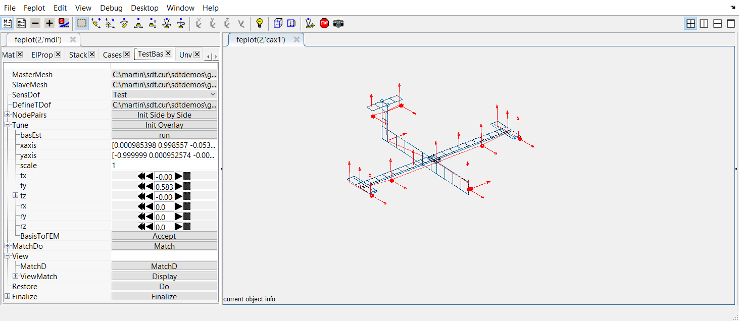
From this better relative position, one needs to iterate manually with small translations tx, ty, tz and rotations rx, ry, rz until the optimum is reached.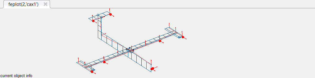
Finally, click on the button Accept associated to BasisToFEM to apply the coordinate transformation to the test wireframe and perform the compute the observation matrix of the FEM at sensors.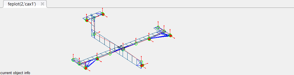
Clicking on Finalize will save the result in the corresponding project. Another strategy using Iterative Closest Point algorithm is also implemented (in the NodePairs sub-table). This will be documented in further release.
In cases where an analytical model of a structure is available before the modal test, it is good practice to use the model to design the sensor/shaker configuration.
Typical objectives for sensor placement are
Sensor placement capabilities are accessed using the fe_sens function as illustrated in the d_cor('TutoSensPlace') demo. This function supports the effective independence [23] and maximum sequence algorithms which seek to provide good placement in terms of modeshape independence.
It is always good practice to verify the orthogonality of FEM modes at sensors using the auto-MAC (whose off-diagonal terms should typically be below 0.1)
cphi = fe_c(mdof,sdof)*mode; ii_mac('cpa',cphi,'mac auto plot')
For shaker placement, you typically want to make sure that
The placement based on the first objective is easily achieved looking at the minimum controllability, the second uses the Multivariate Mode Indicator function (see ii_mmif). Appropriate calls are illustrated in the d_cor('TutoSensPlace') demo.
