PDF Index
| SDT-visc
Contents
Functions
PDF Index |
Even though, viscoelastic constitutive laws are fully characterized by the measurement of a complex modulus. As will be detailed in the next chapter, numerical solvers are often associated with specific analytical representations of moduli. This section illustrates the main classes of modulus representations.
At each frequency, the complex modulus describes an elliptical stress/strain relation. For є=Re(eiω t), one has σ(t)=Re(Es(1+iη)eiω t)=Es(cosω t−ηsinω t) as shown in figure 1.1. One calls, storage modulus the real part of the complex modulus Es=Re(E) and loss factor the ratio of the imaginary and real parts η=Im(E)/Re(E). The loss factor can also be computed as the ratio of the power dissipated over a cycle, divided by 2π by the maximum strain energy
| (1.3) |
This definition in terms of dissipated energy extends the complex modulus definition to cases with small non linearities. In such cases, the dissipation may be a structural rather than a material effect and may depend on amplitude or history so that its use as a constitutive parameters may not be relevant.
The raw measure of viscoelastic characteristics gives a complex modulus which typically has the characteristics shown in figure 1.2.
The solution of frequency domain problems (frequency response functions, complex mode extraction) requires the interpolation of measurements between frequency points (shown as a solid line) and the extrapolation in unmeasured low and high frequency areas (shown in dotted lines in the figure).
For interpolation, a moving average, weighted for 2 or 3 experimental points, is easily implemented and fast to compute. For extrapolation at low frequencies, one will assume a real asymptote E(0) (i.e. η(0)=0) from basic principles : since the relaxation function is real, its Fourier transform is even and thus real at 0. For high frequencies, one uses a complex asymptote E∞,η∞. There are mathematical limitations, on possible values for this asymptote but in practice, there are also other physical dissipation mechanisms that are not represented by the viscoelastic law so that the real objective is to avoid numerical pathologies when pushing the model outside its range of validity.
The main advantage of non parametric representations of constitutive laws is to allow fully general accounting of behavior that are strongly dependent on frequency, temperature, pre-stress, ... Moreover, the direct use of experimental data avoids standard steps of selecting a representation and identifying the associated parameters. Since good software to perform those steps is not widespread, avoiding them is really useful.
Disadvantages are very few and really mostly linked to the extraction of complex modes and as a consequence time response simulations using modal bases. And even these difficulties can be circumvented.
The classical approach in rheology is to represent the stress/strain relation as a series of springs and viscous dashpots. Figure 1.3 shows the simplest models [3].
Maxwell's model is composed of a spring and a dashpot in series. Each element carries the same load while strains are added. The stress / strain relation is, in the frequency domain, written as
| (1.4) |
where
| (1.5) |
is a settling time that is characteristic of the model and is associated to a pole at ω=−E/C = −1/τ.
The viscous model, called Kelvin Voigt Model, is composed of a spring and a dashpot in parallel. Each element undergoes the same elongation but strains add. Damping is then represented by the addition of strains proportional to deformation and deformation velocity. In the frequency domain the modulus has the form
| (1.6) |
Structural damping, also called hysteretic damping, is introduced by considering a complex stiffness that is frequency independent. The complex modulus is thus characterized by constant storage moduli and loss factors
| (1.7) |
The standard viscoelastic solid has a constitutive law given by
| (1.8) |
leading to a time domain representation
| (1.9) |
Figure 1.4 shows the frequency domain properties of these models. Maxwell's model is only valid in the high frequency range since its static stiffness is zero. The viscous damping model is unrealistic because the loss factor goes to infinity at high frequency (there deformation locking).
The structural damping model approximates the modulus by a complex constant. Although it does not represent accurately any viscoelastic material, such as the one shown in figure 1.2, it leads to a good approximation when the global behavior of the structure is not very sensitive to the evolution of the complex modulus with frequency. This model is generally adapted for materials with load damping (metals, concrete, ...).
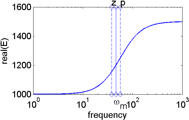
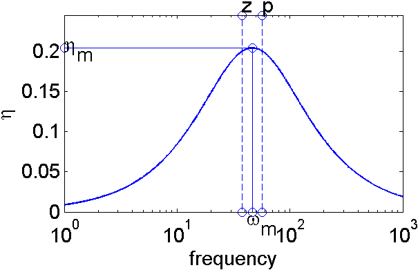
The standard viscoelastic model has the main characteristics of real materials : low and high frequency asymptotes, maximum dissipation at the point of highest slope of the real part of the modulus.
This model is characterized a nominal level E0 and two pairs of related quantities: a pole
| (1.10) |
where the modulus flattens out, and a zero
| (1.11) |
giving the inflection point where the modulus starts to augment; or the maximum loss factor
| (1.12) |
and the frequency where this maximum is reached (between the pole and the zero)
| (1.13) |
The maximum loss factor is higher when the pole and zero are well separated and the low and high frequency moduli differ. This is consistent with the fact that materials that dissipate well also have storage moduli that are strongly frequency dependent.
Figure 1.6 illustrates problems encountered with three parameter models. The parameters of the standard viscoelastic model where chosen to match the low and high frequency asymptote and the frequency of the maximum in the loss factor. One clearly sees that the slope is not accurately represented and more importantly that the loss factor maximum and evolution in frequency are incorrect. These limitations have motivated the introduction of more complex models detailed in the following sections.
The first generalization is the introduction of higher order models in the form of rational fractions. All classical representations of rational fractions have been considered in the literature. Thus, fractions of high order polynomials, decompositions in products of first order polynomials giving poles and zeros, sums of low order fractions
| (1.14) |
are just a few of various equivalent representations.
Figure 1.7 shows two classical representations. Maxwell generalized model introduces a pole (λj=Ej/Cj, associated to settling time τj=Cj/Ej) and high frequency stiffness Ej for each spring/dashpot branch.
The physical meaning of each representation is identical. However, each representation may have advantages when posing equations for implementation in a numerical solver. damp12.bib Refs. citebal43 discusses models using particular representations of the modulus of order 2 (so called GHM models for Golla, Hughes, McTavish [4, 5]) and order 1 (so called ADF models for Anelastic Displacement Field [6, 7, 8]). These are shown to correspond to the formalism of materials with internal states that are commonly used in non linear mechanics. The PhD of F. Renaud [] is an example of recent work on this issue. For example, section 2.2.3 will discuss models using particular representations of the modulus of order 2 (so called GHM models for Golla, Hughes, McTavish [4, 5]) and order 1 (so called ADF models for Anelastic Displacement Field [6, 7, 8]). This section will also show how these models correspond to the formalism of materials with internal states that are commonly used in non linear mechanics.
Rational fractions have a number of well known properties. In particular, the modulus slope at a given frequency s=iω is directly characterized by the position of poles and zeros in the complex plane (see Bode diagram building rules in any course in controls [9]). The modulus slopes found in true materials are generally such that it is necessary to introduce at least one pole per decade to accurately approximate experimental measurements (see [10] for a discussion of possible identification strategies). This motivated the use of fractional derivatives described in the next section.
The use of non integer fractions of s allows a frequency domain representation with an arbitrary slope. A four parameter model is thus proposed in [11]
| (1.15) |
where the high Einf and low Emin=g0*Einf frequency moduli are readily determined and the ω and α coefficients are used to match the frequency of the maximum loss factor and its value. Properties of this model are detailed in [2].
One can of course use higher order fractional derivative models. To formulate constant matrix models one is however bound to use rational exponents damp12.bib(see [](see section 2.2.4).
The main interest of fractional derivative models is to allow fairly good approximations of realistic material behavior with a low number of parameters. The main difficulty is that their time representation involves a convolution product. One will find in Ref. [12] an analysis of the thermomechanical properties of fractional derivative models as well as a fairly complete bibliography.
It is often necessary to split constitutive laws. This is done in fevisco MatSplit. For isotropic materials the usual law
| (1.16) |
with at nominal G=E/(2(1+ν)). But in reality the bulk modulus K=E./(3*(1−2ν)) is not very damped and does not decrease notably with temperature while G is much more sensitive.
| (1.17) |