4.1 Rigid disk example
| Figure 4.1: Simple rigid disk. |
We consider a simple rigid disk of axis Y, thickness h, radius R, mass m. This simple example is very useful because we can easily compute matrices in both of global and local frame for a simple description of motion with 4 DOF. Besides we can compute in SDT equivalent matrices for a mass1 rigid disk, for a disk described by a beam1 element and for a volume disk in hexa8 elements. Then we can compare gyroscopic matrices and make sure that their implementation for each element is correct.
4.1.1 Matrices in rotating frame
The motion of the disk is described by 2 translations (uc and wc) and 2 rotations DOF (θu and θw).
Disk is assumed to be rigid so displacements at each point of the disk are given by the shape functions
Rotation matrix (2.3) along Y axis is given by
Using matrix expression given in section 2.1.1 in body fixed local rotating frame, and projecting the integrals by assuming rigid disk motion
with Iu=Iw=1/4mR2+mh2/12
An unbalanced mass is represented by a static load in the local rotating frame
4.1.2 Matrices in global fixed frame
Local frame (indexed with L) is rotating in global fixed frame (indexed with G) according to rotation matrix
so that we have
{qL}=[Rt]{qG}
{qL}=[Rt] {qG}+[Ṙt] {qG}
{ qL}=[Rt] { qG}+2[Ṙt]{qG}+[ Rt] {qG}
and equation (4.6) can thus be rewritten as
One has RT Ṙ=Ω [
] and RT R=Ω2 [
] thus in the gyroscopic effect the translation terms disappear and one has
with Iv=1/4mR2=Iu−2mh2/12 and the xxx UNEXPECTED xxx centrifugal softening in the global frame
An unbalanced mass is represented by a rotating load in the global fixed frame
4.1.3 Validation with 3D model disk
This validation example considers a disk meshed with hexa8 volume elements.
Local frame matrices are computed and projected on the geometrical rigid body modes (x and z translations, and corresponding rotation). One checks matching of
-
matching of theoretical and numerical matrices
- response amplitudes of the disk with unbalanced mass in global and local frame
- mass1 and beam1 elements gives the same gyroscopic matrices in the global frame (mattype 70)
R1=.01;R2=.15;h=0.03;rho=7800;
md=d_rotor(sprintf('testvoldisk -dim %.15g %.15g %.15g 5 24',R1,R2,h))
md.DOF=[];md=fe_caseg('assemble -se -matdes 2 1 7 8 not',md);
rb=feutil('geomrb',md); cf=feplot(md); cf.def=rb;
md.K=feutil('tkt',rb.def(:,[1 3 4 6]),md.K);
md.DOF=[1.01 1.03 1.04 1.06]';
md.K{2}=0*md.K{2};
md.K{2}(1,1)=5e5;md.K{2}(2,2)=5e5;
md.K{2}(3,3)=1e5;md.K{2}(4,4)=1e5;
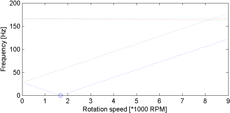
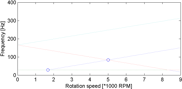
fe_rotor('campbell-critical',md,linspace(0,9000,31));
w=1; t=12; wrange=logspace(0,3,100); Q=[];
for j1=1:length(wrange);w=wrange(j1);
R=[cos(w*t) -sin(w*t); sin(w*t) cos(w*t)]; R=[R zeros(2);zeros(2) R];
Rp=w*[-sin(w*t) -cos(w*t); cos(w*t) -sin(w*t)];Rp=[Rp zeros(2);zeros(2) Rp];
Rpp=-w^2*R;
MG=R'*md.K{1}*R;
DG=2*R'*md.K{1}*Rp + R'*w*md.K{3}*R;
KG=R'*md.K{1}*Rpp + R'*w*md.K{3}*Rp + R'*w^2*md.K{4}*R + R'*md.K{2}*R;
m=pi*(R2^2-R1^2)*3e-2*7800;
Iv=0.5*m*(R2^2+R1^2); Iu=0.5*Iv+m*h^2/12;
DGth=zeros(4); DGth(4,3)=Iv; DGth(3,4)=-Iv; DGth=w*DGth;
KGth=diag([0 0 1 1]); KGth=-w^2*Iv/2*KGth;
if norm(KG-R'*md.K{2}*R-KGth)/norm(KGth)>5e-2;error('Cent. soft mismatch');end
if norm(DG-DGth)/norm(DGth)>5e-2; error('gyro matrix mismatch'); end
X0L=inv(md.K{2}+w^2*md.K{4})*w^2*[1 0 0 0]';
X0L=abs(X0L(1));
X0G=inv(-w^2*MG+1i*w*DG+KG) *w^2*[-1i 1 0 0]';
X0G=abs(X0G(1));
Q(1,j1)=X0L; Q(2,j1)=X0G;
end
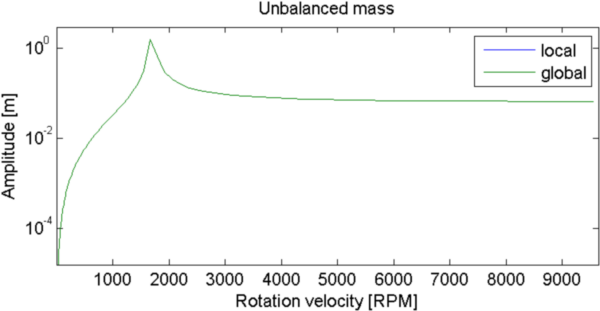
figure(4);semilogy(wrange*60/2/pi,Q(1,:),wrange*60/2/pi,Q(2,:));
legend('local','global'); title('Unbalanced mass');setlines
xlabel('Rotation velocity [RPM]'); ylabel('Amplitude [m]')
if norm(Q(1,:)-Q(2,:))/norm(Q(1,:))>1e-8; error('Global/Local error'); end
mdmass=struct('Node',[1 0 0 0 0 0 0], ...
'Elt',[Inf abs('mass1') 0; 1 m m m Iu Iv Iu]);
mdmass=fe_case(mdmass,'fixdof','Base',[1.02 ;1.05])
mdmass=fe_caseg('assemble -se -matdes 2 1 70',mdmass)
if norm(w*mdmass.K{3}-DGth)/norm(DGth)>1e-8; sdtw('_err','mass1 gyro 70 unmatch'); end
Omega=[0 1 0];
mdbeam1=struct('Node',[1 0 0 0 -h/2*Omega; 2 0 0 0 h/2*Omega],...
'Elt',[Inf abs('beam1') 0; 1 2 1 1 0 0 0]);
mdbeam1.il=p_beam('convertto1',p_beam(sprintf('dbval 1 TUBE %.15g %.15g',R2,R1)));
mdbeam1.pl=m_elastic('dbval 1 steel');
mdbeam1=fe_case(mdbeam1,'fixdof','fix1',...
[1+(find(Omega)+[0;3])/100;2+(find(Omega)+[0;3])/100]);
rb=feutil('geomrb',mdbeam1); mdbeam1=fe_case(mdbeam1,'DofSet','fix2',rb);
rb=fe_simul('static',mdbeam1); mdbeam1=fe_case(mdbeam1,'remove','fix2');
mdbeam1.DOF=[]; mdbeam1=fe_caseg('assemble -se -matdes 2 1 70',mdbeam1);
mdbeam1.DOF=fe_case('gettdof',mdbeam1);
rb=feutil('placeindof',mdbeam1.DOF,rb)
mdbeam1.K=feutil('TKT',rb.def(:,setdiff(1:6,find(Omega)+[0 3])),mdbeam1.K)
if norm(w*mdbeam1.K{3}-DGth)/norm(DGth)>1e-8;
sdtw('_err','beam1 gyro 70 unmatch');
end
The response to the unbalanced mass is the same in both of the 2 frames.
The maximum of response matches rotation speed found as critical speed for forward whirl in local and global Campbell diagram.
Note that we can compute Campbell in local frame from Campbell in global frame with:
fL(F)=||fG(F)−Ω|| for forward modes and
fL(B)=||fG(B)+Ω|| for backward modes.
The 2 Campbell diagrams have been computed using matrices in corresponding frame and we check that we can pass from one to other using these formulas.
XXX In this example:
- Centrifugal softening in global fixed frame? Not 0
- In GLOBAL frame gyroscopic matrix DG do not modify unbalanced response because only translation dof are affected...
- In LOCAL frame gyroscopic D do not modify unbalanced response:
X0L=inv(md.K2+w2*md.K4)*w2*[1 0 0 0]'; % local
| Figure 4.2: Top: Unbalanced mass response amplitude computed in local and global frame. Bottom left: Campbell diagram in local rotating frame, right: in global frame. |
©1991-2023 by SDTools