PDF Index
| SDT-piezo
Contents
Functions
PDF Index |
This example deals with an aluminum plate with 4 piezoceramic patches. The geometry is the one presented in Section 2.1, Figure 2.1. It corresponds to a cantilevered plate with 4 piezoelectric patches modeled using the p_piezo Shell formulation.
The first step consists in the creation of the model, the definition of the boundary conditions, and the definition of the default damping coefficient.
( d_piezo('TutoPlate_4pzt_single-s1')
)
The resulting mesh is shown in Figure 2.10, in Section 2.1, where the different possible approaches to build the mesh are discussed in details.
d_piezo('TutoPlate_4pzt_single-s1')
)
The resulting mesh is shown in Figure 2.10, in Section 2.1, where the different possible approaches to build the mesh are discussed in details.
% See full example as MATLAB code in d_piezo('ScriptTutoPlate_4pzt_single')
%% Step 1 - Build model and visualize
model=d_piezo('MeshULBplate');  % creates the model
model=fe_case(model,'FixDof','Cantilever','x==0'); % Clamp plate
% Set modal default zeta = 0.01
model=stack_set(model,'info','DefaultZeta',0.01);
cf=feplot(model); fecom('colordatagroup'); set(gca,'cameraupvector',[0 1 0])
One can have access to the piezoelectric material properties and the list of nodes associated to each pair of electrodes. Here nodes 1055 to 1058 are associated to the four pairs of electrodes defined in the model. The corresponding degree of freedom is the difference of potential between the electrodes in each pair corresponding to a specific piezoelectric layer. In this models, layers 1 and 3 are piezoelectric in groups 2 and 3 (the internal layer correspond to supporting aluminum plate). Therefore only .21 (electrical) DOF is associated to nodes 1055-1058.
p_piezo('TabDD',model);      % List piezo constitutive laws
r1=p_piezo('TabInfo',model); % List piezo related properties
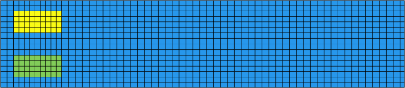
Figure 2.10: Mesh of the composite plate. The different colours represent the different groups
The next step consists in the definition of the actuators and sensors in the model. Here, we consider one actuator on Node 1055 (layer 1 of group 1), the four piezoelectric patches are used as charge sensors, and the tip displacement of the cantilever beam is measured at the right-upward corner of the beam (corresponding to node 1054 here). Note that in
order for Q-S1, Q-S2 and Q-S3 to measure resultant charge, the corresponding electrical difference of potential needs to be set to zero. If this
is not done, then the charge sensors will measure a charge close to zero (round-off errors) as there is no charge when the difference of potential
across the electrodes is free. For Q-Act, the electrical dof is already fixed due to the fact that the patch is used as a voltage actuator.
(d_piezo('TutoPlate_4pzt_single-s2')
)
%% Step 2 - Define actuators and sensors
nd=feutil('find node x==463 & y==100',model);
model=fe_case(model,'SensDof','Tip',nd+.03); % Displ sensor
i1=p_piezo('TabInfo',model);i1=i1.Electrodes(:,1);
model=fe_case(model,'DofSet','V-Act',struct('def',1,'DOF',i1(1)+.21)); %Act
model=p_piezo(sprintf('ElectrodeSensQ  %i Q-Act',i1(1)),model); % Charge sensors
model=p_piezo(sprintf('ElectrodeSensQ  %i Q-S1',i1(2)),model);
model=p_piezo(sprintf('ElectrodeSensQ  %i Q-S2',i1(3)),model);
model=p_piezo(sprintf('ElectrodeSensQ  %i Q-S3',i1(4)),model);
% Fix ElectrodeSensQ dofs to measure resultant (charge)
model=fe_case(model,'FixDof','SC*S1-S3',i1(2:end)+.21);
sens=fe_case(model,'sens');
In order to check the effect of the actuator, we compute the static response using the full model and represent the deformed shape (Figure 2.11).
(d_piezo('TutoPlate_4pzt_single-s3')
)
%% Step 3 Compute static and dynamic response
d0=fe_simul('dfrf',stack_set(model,'info','Freq',0)); % direct refer frf at 0Hz
cf.def=d0; fecom(';view3;scd 20;colordatagroup;undefline')
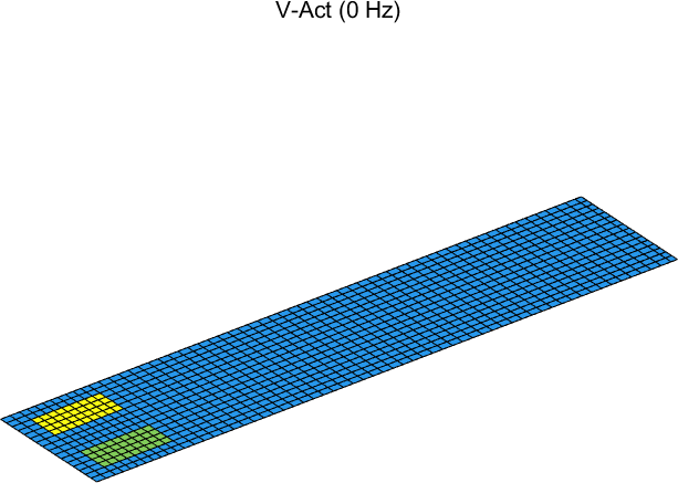
Figure 2.11: Deformed shape under voltage actuation on one of the bottom piezoelectric patches
We can now compute the transfer function between the actuator and the four charge sensors, as well as the tip sensor using the full model. The result is stored in the variable C1.
% Compute frequency response function (full model)
if sdtkey('cvsnum','mklserv_client')>=126;ofact('mklserv_utils -silent')
    f=linspace(1,100,400); % in Hz
else;
  f=linspace(1,100,100); % in Hz (just 100 points to make it fast)
end

d1=fe_simul('dfrf',stack_set(model,'info','Freq',f(:))); % direct refer frf
% Project response on sensors
C1=fe_case('SensObserve -DimPos 2 3 1',sens,d1);C1.name='DFRF';C1.Ylab='V-Act';
C1.Xlab{1}={'Frequency','Hz'};
A reduced state-space model can be built and the frequency response function calculated, and stored in the variable C2. The two curves obtained are compared to show the accuracy of the reduced state-space model in Figure 2.12.
(d_piezo('TutoPlate_4pzt_single-s4')
)
%% Step 4 - Build state-space model
[s1,TR1]=fe2ss('free 5 10 0',model); %
C2=qbode(s1,f(:)*2*pi,'struct');C2.name='SS';

% Compare the two curves
ci=iiplot;
iicom(ci,'curveinit',{'curve',C1.name,C1;'curve',C2.name,C2});
iicom('submagpha');
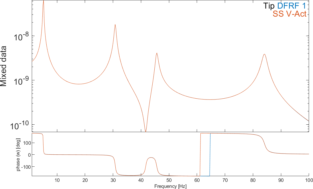
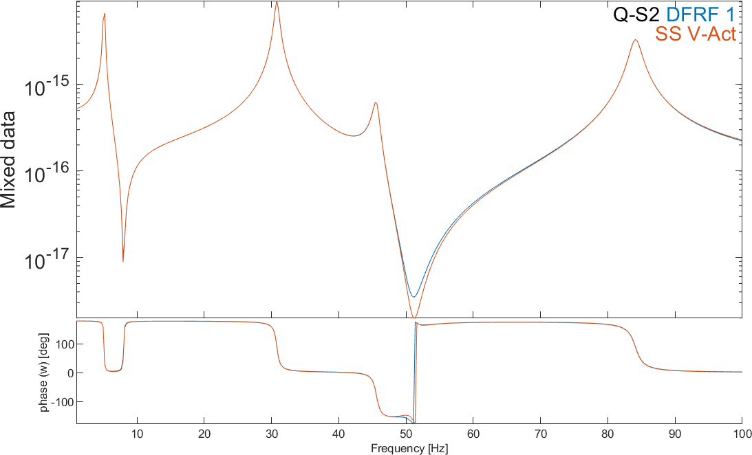
Figure 2.12: Comparison of FRF due to voltage actuation with the bottom piezo: full (DFRF) and reduced (SS) state-space models. Tip displacement and charge corresponding to electrical node 1682
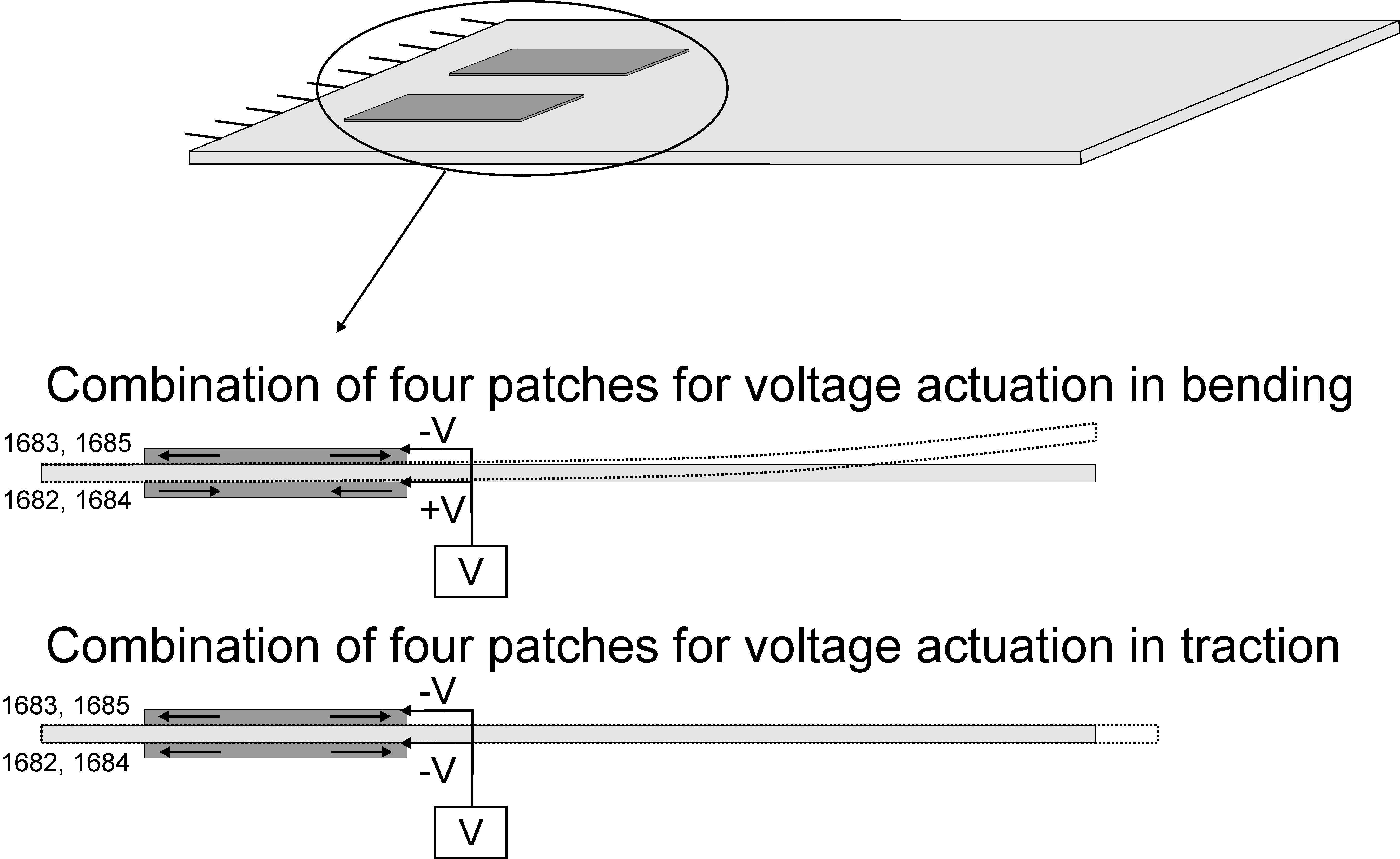
Combination of electrodes can be used in order to build a variety of actuators and sensors. For example, using the four piezoelectric patches, it is possible to induce a pure bending in the cantilever plate by using the following combination: the two actuators on one side of the plate are combined (the same voltage is applied to both simultaneously), while the two actuators on the opposite side are combined and driven out of phase. This allows to cancel the in-plane effect of the patches and to induce a pure bending. If all 4 actuators are driven in phase, then it only induces in-plane forces causing displacements only in the plane of the plate (Figure 2.13).
The corresponding script to combine all four patches for bending and traction is:
(d_piezo('TutoPlate_4pzt_comb-s1')
)
% See full example as MATLAB code in d_piezo('ScriptTutoPlate_4pzt_Comb1')
%% Step 1 - Build model and define actuator combinations
model=d_piezo('MeshULBplate -cantilever');  % creates the model
model=stack_set(model,'info','DefaultZeta',0.01); % Set modal damping zeta = 0.01

% combine electrodes to generate pure bending / pure traction
data.def=[1 -1 1 -1;1 1 1 1]'; % Define combinations for actuators
data.lab={'V-bend';'V-Tract'};
data.DOF=p_piezo('electrodeDOF.*',model);
model=fe_case(model,'DofSet','V_{In}',data);
(d_piezo('TutoPlate_4pzt_comb-s2')
)
%% Step 2 Compute static response
d0=fe_simul('dfrf',stack_set(model,'info','Freq',0)); % direct refer frf
cf=feplot(model); cf.def=d0;
fecom(';view3;scd .02;colordataEvalZ;undefline')
The resulting static deflections of the plate are shown in Figure 2.14.
.png)
.png)
Figure 2.14: Static responses using a combination of actuators in order to induce pure bending or pure in-plane motion
We can now define two displacements sensors at the tip in the z and x directions and compute the FRFs between the bending actuator and the two displacements as well as the traction actuator and the two displacement sensors (Figure 2.15). The bending actuator/'Tip-z' FRF show three resonances corresponding to the first three bending mode shapes, while the traction actuator/'Tip-x' FRF shows no resonance due to the fact that the traction mode shape has a frequency much higher than the frequency band of the calculations. The FRFs show clearly the possibility to excite either bending or traction independently on the plate. The two other FRFs are close to zero.
(d_piezo('TutoPlate_4pzt_comb-s3')
)
%% Step 3 - Dynamic response and state-space model
% Add tip displacement sensor in x and z
nd=feutil('find node x==463 & y==100',model);
model=fe_case(model,'SensDof','Tip-z',nd+.03); % Z-disp
model=fe_case(model,'SensDof','Tip-x',nd+.01); % X-disp

% Make SS model and display FRF
[sys,TR]=fe2ss('free 5 30 0 -dterm',model);
C1=qbode(sys,linspace(1,100,400)'*2*pi,'struct');
C1.name='Bend-tract combination'; % Force name
C1.X{2}={'Tip-z';'Tip-x'}; % Force input labels
C1.X{3}={'V-bend';'V-tract'}; % Force output labels
iicom('CurveReset');iicom('curveinit',C1)
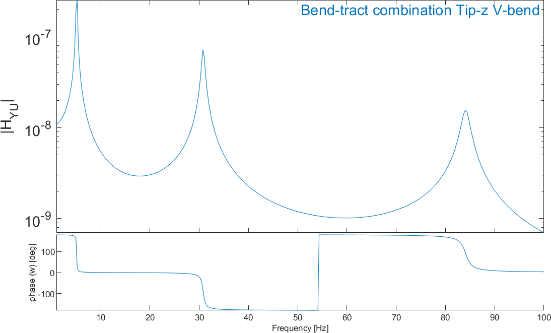
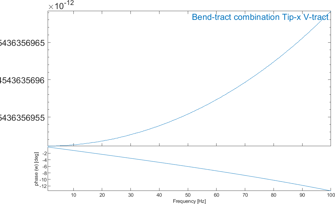
Figure 2.15: Bending actuator/'Tip-z' FRF (left) and traction actuator/'Tip-x' FRF (right)
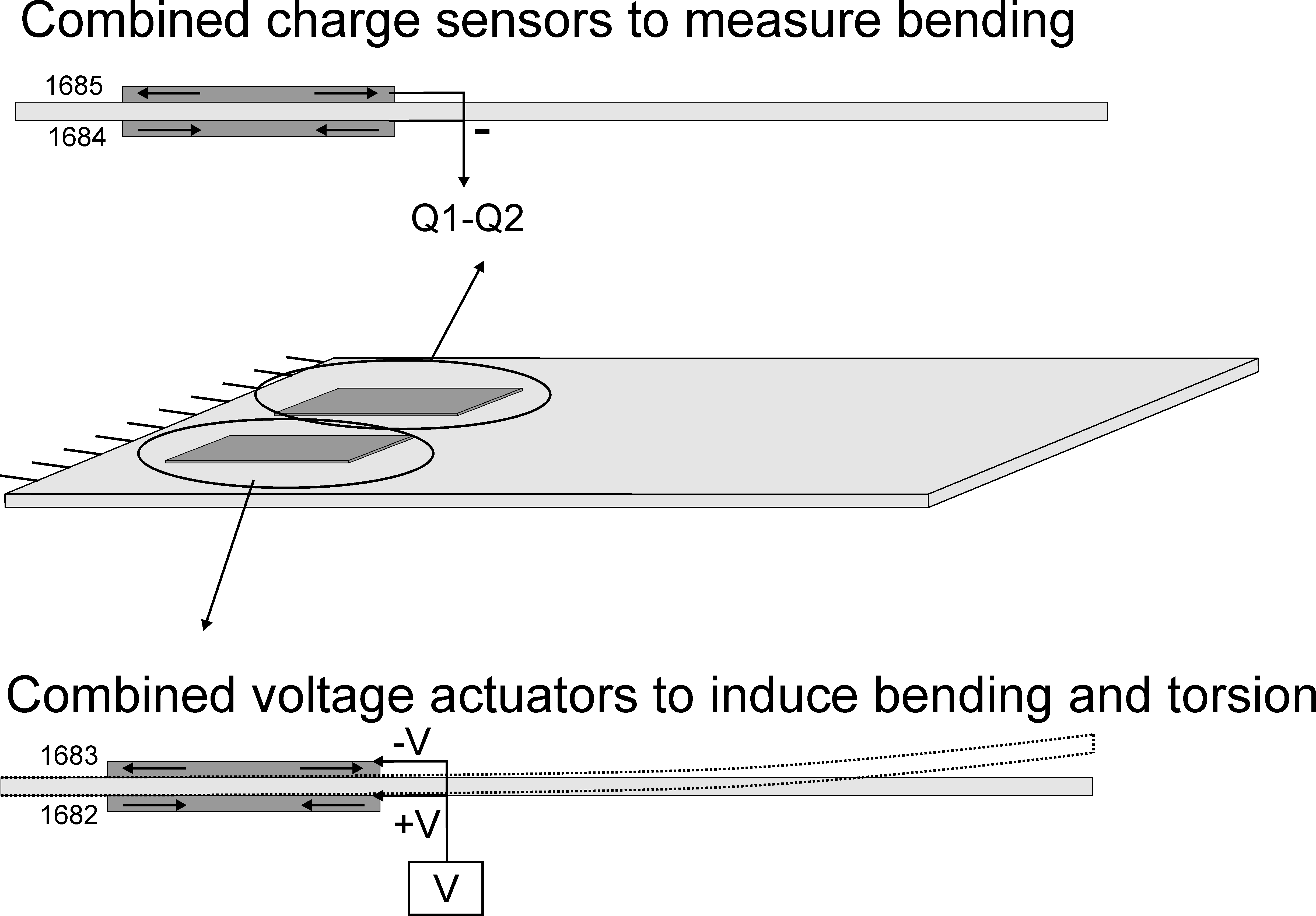
Voltage and charge sensors can also be combined. Let us consider a voltage combination of nodes 1055 and 1056 for actuation, which will result in bending and a slight torsion of the plate due to the unsymmetrical bending actuation.
(d_piezo('TutoPlate_pzcomb_2-s1')
)
% See full example as MATLAB code in d_piezo('ScriptTutoPlate_4pzt_Comb2')
%% Step 1 - Build model and define actuator combinations
model=d_piezo('MeshULBplate cantilever');  % creates the model
model=stack_set(model,'info','DefaultZeta',0.01); % Set modal damping zeta = 0.01
edofs=p_piezo('electrodeDOF.*',model);
model=fe_case(model,'DofSet','V1+2', ...
    struct('def',[1;-1],'DOF',edofs(1:2)));
(d_piezo('TutoPlate_pzcomb_2-s2')
)
%% Step 2 - Compute static response
d0=fe_simul('dfrf',stack_set(model,'info','Freq',0)); % direct refer frf
cf=feplot(model); cf.def=d0;
fecom(';view3;scd .1;colordatagroup;undefline')
We now define two sensors, consisting in charge combination with opposite signs for nodes 1057 and 1058
and voltage combination with opposite signs for the same nodes (Figure 2.16 shows the case of charge combination).
(d_piezo('TutoPlate_pzcomb_2-s3')
)
%% Step 3 - Define sensor combinations
% Combined charge output (SC electrodes) % difference of charge 1684-1685
r1=struct('cta',[1 -1],'DOF',edofs(3:4),'name','QS3+4');
model=p_piezo('ElectrodeSensQ',model,r1);
% Combined voltage output (OC electrodes) % difference of voltage 1684-1685
r1=struct('cta',[1 -1],'DOF',edofs(3:4),'name','VS3+4');
model=fe_case(model,'SensDof',r1.name,r1);
model=fe_case(model,'pcond','Piezo','d_piezo(''Pcond 1e8'')');
By default, the electrodes are in 'open-circuit' condition for sensors, except if the sensor is also used as voltage
actuator which corresponds to a 'short-circuit' condition. Therefore, as the voltage is left 'free' on nodes 1057 and 1058,
the charge is zero and the combination will also be zero. If we wish to use the patches as charge sensors, we need to
short-circuit the electrodes, which will result in a zero voltage and in a measurable charge. This is illustrated by
computing the response in both configurations (open-circuit by default, and short-circuiting the electrodes for nodes 1057 and
1058):
(d_piezo('TutoPlate_pzcomb_2-s4')
)
%% Step 4 - Compute dynamic response with state-space model
[sys,TR]=fe2ss('free 5 10 0 -dterm',model);
 C1=qbode(sys,linspace(1,100,400)'*2*pi,'struct'); C1.name='OC';

% Now you need to SC 1057 and 1058 to measure charge resultant
model=fe_case(model,'FixDof','SC*3-4',edofs(3:4));
[sys2,TR2]=fe2ss('free 5 10 0 -dterm',model);
C2=qbode(sys2,linspace(1,100,400)'*2*pi,'struct');C2.name='SC';

% invert channels and scale
C1.Y=fliplr(C1.Y); C1.X{2}= flipud(C1.X{2});
C2.Y(:,1)=C2.Y(:,1)*C1.Y(1,1)/C2.Y(1,1);
iicom('curvereset'),iicom('curveinit',{'curve',C1.name,C1;'curve',C2.name,C2 });
The FRF for the combination of charge sensors is not exactly zero but has a negligible value in the 'open-circuit' condition, while the voltage
combination is equal to zero in the 'short-circuit' condition. Charge sensing in the short-circuit condition and voltage sensing in the open-circuit condition are compared by scaling the two FRFs to the static response (f=0 Hz) and the result is shown on Figure 2.17. The FRFs are very similar but the eigenfrequencies are slightly lower in the case of charge sensing. This is due to the well-known fact that open-circuit always
leads to a stiffening of the piezoelectric material. The effect on the natural frequency is however not very strong due to the small size of the piezoelectric patches with respect to the full plate.
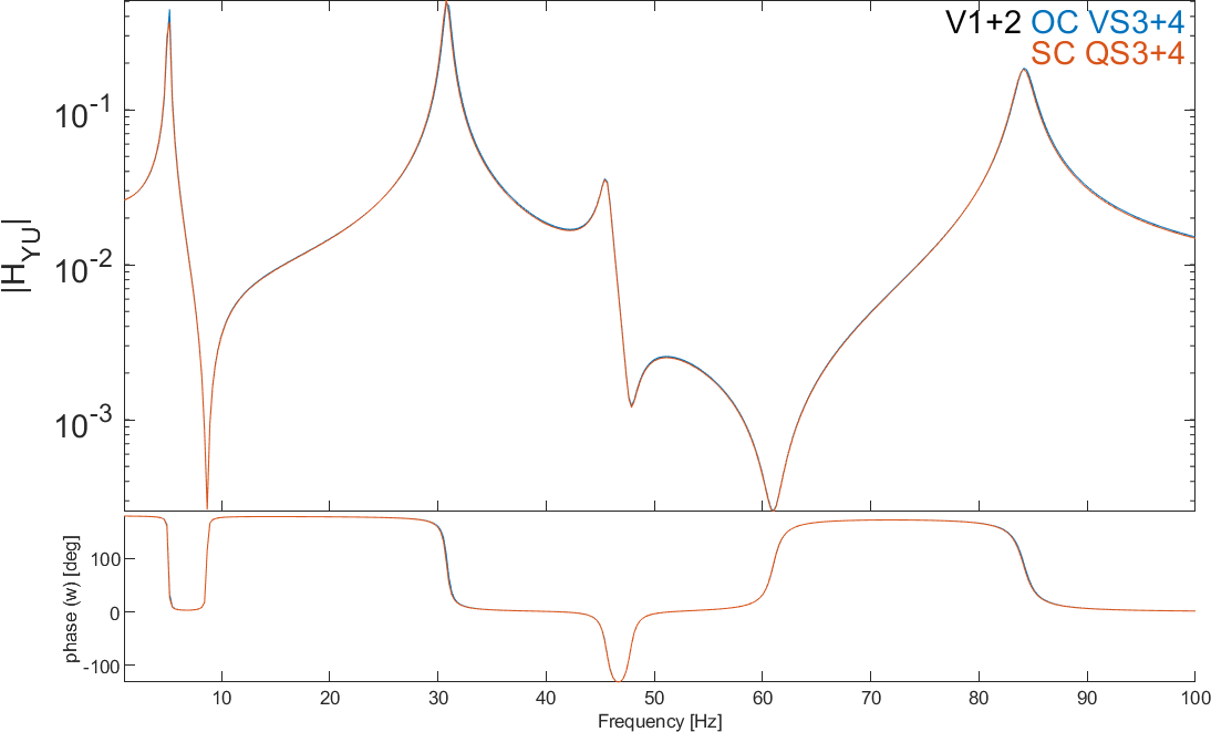
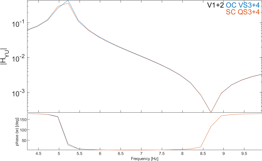
Figure 2.17: Comparison of FRFs (scaled to the static response) for voltage (green) and charge (blue) sensing. Zoom on the third eigenfrequency (right)
The stiffening effect due to the presence of an electric field in the piezoelectric material when the electrodes are in the open-circuit condition is a consequence of the piezoelectric coupling. One can look at the level of this piezoelectric coupling by comparing the modal frequencies with the electrodes in open and short-circuit conditions.
(d_piezo('TutoPlate_pzcomb_2-s5')
)
%% Step 5 - Compute OC and SC frequencies
model=d_piezo('MeshULBplate -cantilever');
% Open circuit : do nothing on electrodes
d1=fe_eig(model,[5 20 1e3]);
% Short circuit : fix all electric DOFs
DOF=p_piezo('electrodeDOF.*',model);
d2=fe_eig(fe_case(model,'FixDof','SC',DOF),[5 20 1e3]);
r1=[d1.data(1:end)./d2.data(1:end)];
plot(r1,'*','linewidth',2);axis tight
xlabel('Mode number');ylabel('f_{OC}/f_{SC}');
Figure 2.18 shows the ratio of the eigenfrequencies in the open-circuit vs short-circuited conditions. The difference depends on the mode number but is always lower than 1%. Higher stiffening effects occur when more of the strain energy is contained in the piezoelectric elements, and the coupling factor is higher.
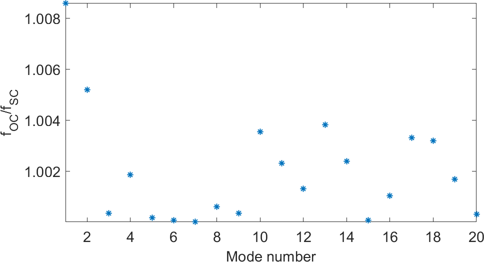
Figure 2.18: Ratio of the natural frequencies of modes 1 to 20 in open-circuit vs short-circuit conditions illustrating the stiffening of the piezoelectric material in the open-circuit condition