SDT-piezo         Contents     Functions              PDF Index

4.2  Collocated force-displacement pairs

Collocated force-displacement pairs are commonly used in active vibration control, as they result in an alternance of poles and zeros in the open-loop transfer functions, leading to unconditionally stable control schemes (when actuators and sensors dynamics are neglected).
The fe_case('DofLoadSensDof') command provides a generic way to build collocated pairs. On first defines the sensors (related to DOFs in the model) and then creates the corresponding collocated forces. This is illustrated In the d_piezo('TutoPzBeamCol') demo below on a 3D model of a U-shaped cantilever beam.
The first step d_piezo('TutoPzBeamCol-s1') consists in the meshing, application of boundary conditions and point sensor definition.

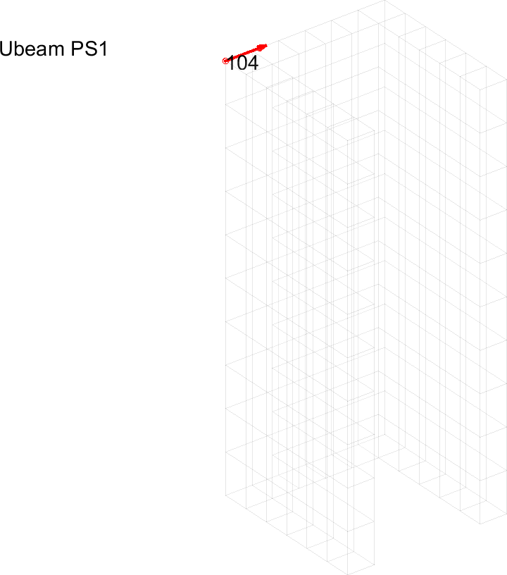
The sensor is defined on node 104 in direction x with the following call.

% Introduce a point displacement sensor and visualize
% sdtweb sensor#slab % URN based definition of sensors
model = fe_case(model,'SensDOF','Point Sensors',{'104:x'});

Figure 4.1 shows the finite element mesh of the U-beam with a sensor added on node 104 in the x-direction. In (d_piezo('TutoPzBeamCol-s2') ), the load is then defined as being collocated to the sensor, i.e, in the x-direction and on node 104 with the following call:

%% Step 2 : Introduce collocated force actuator and compute response
model=fe_case(model,'DofLoad SensDof','Collocated Force','Point Sensors:1') 
% 1 for first sensor if there are multiple

The static response of the U-beam to this load is computed with fe_simul and shown in Figure 4.2.

---

Figure 4.1: U-beam with displacement sensor added on node 104 in direction x

---

---

Figure 4.2: Static response of U-beam to load on node 104 in direction x

---

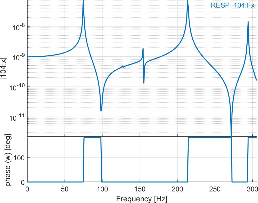
In d_piezo('TutoPzBeamCol-s3') , the collocated transfer function is then computed using fe_simul and plotted in the iiplot environment (Figure 4.3).

---

Figure 4.3: Collocated transfer function for a force applied on node 104 in direction x, and a displacement at the same node and in the same direction

---

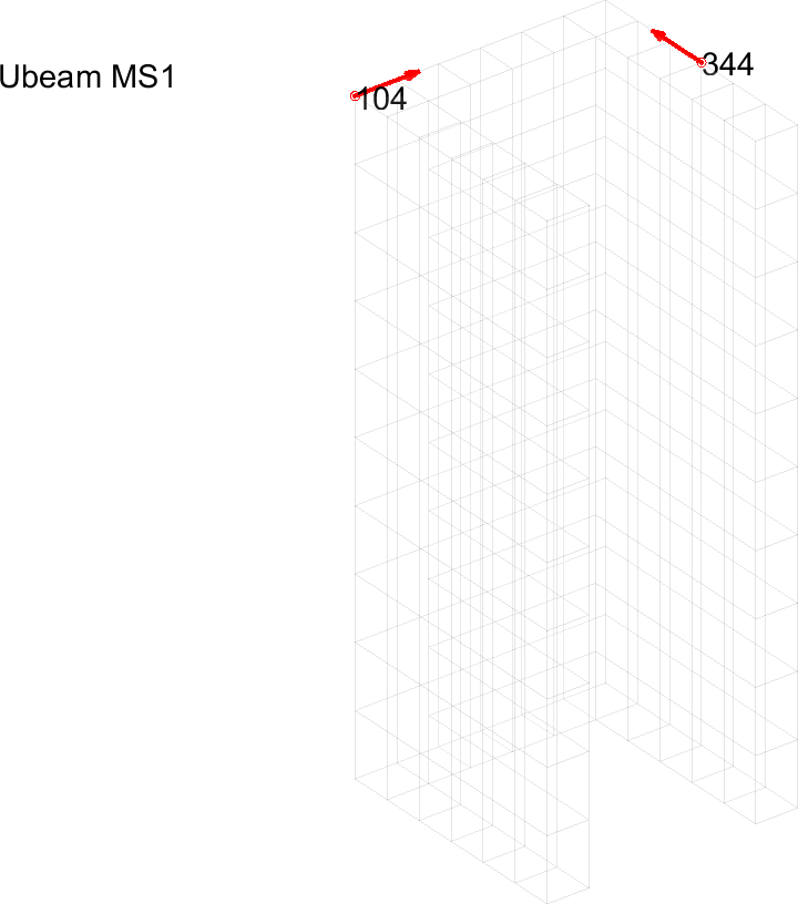
Multiple sensors and actuators can also be generated. In d_piezo('TutoPzBeamCol-s4') , the single sensor is changed to two sensors (adding a sensor on node 344 in y-direction). Note that if the same name is used in the definition of the sensors, the previous definition is replaced (here 'Point sensors' is the name of the sensing case). The two sensors are shown on Figure 4.4.

%% Step 4 : multiple collocated sensors and actuators
% Introduce two sensors and visualize
model = fe_case(model,'SensDOF','Point sensors',{'104:x';'344:y'});
cf=feplot(model);

---

Figure 4.4: U-beam with displacement sensor added on node 104 in direction x and 344 in direction y

---

Two forces collocated to these sensors are then defined in d_piezo('TutoPzBeamCol-s5') , and the static response is computed and shown in Figure 4.5.
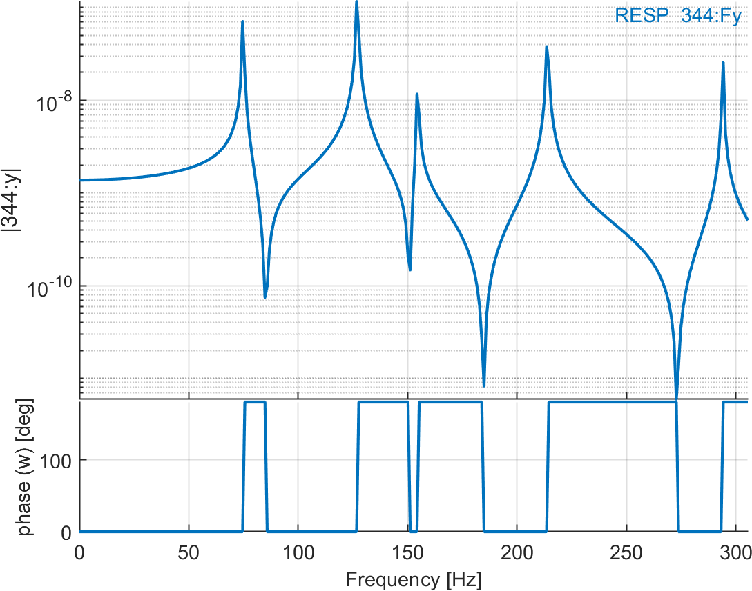
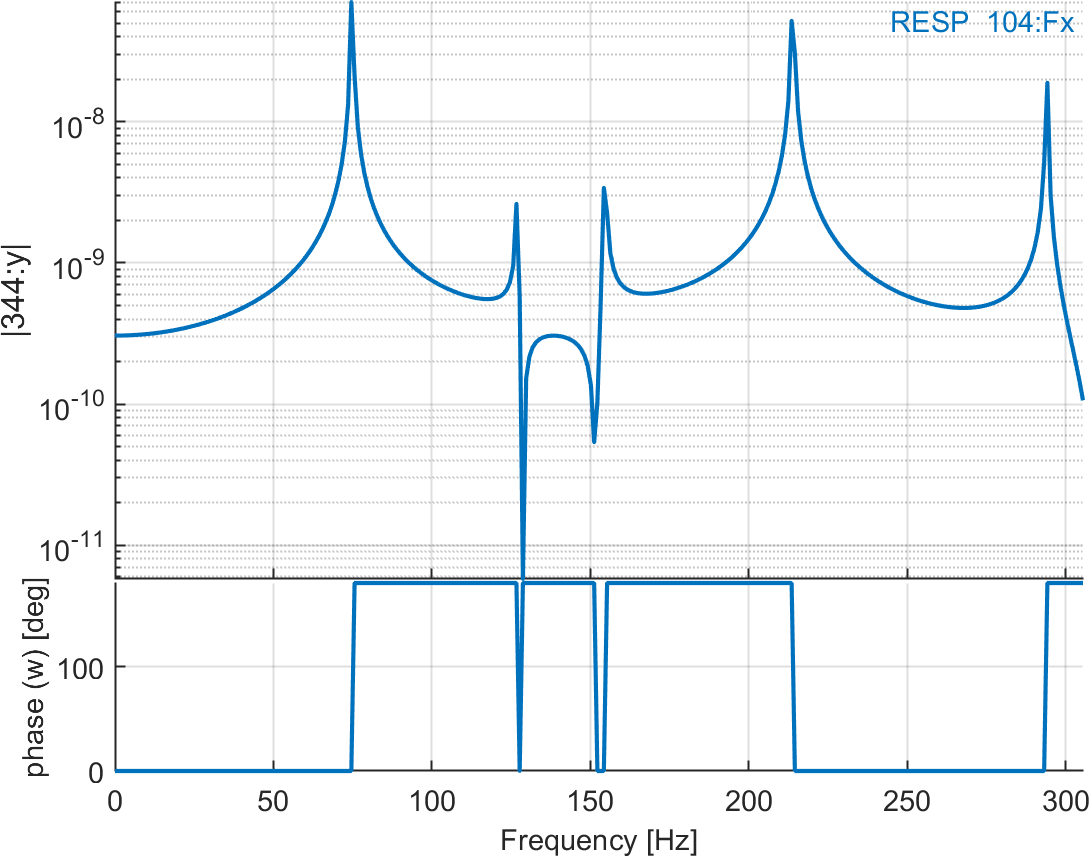
The four transfer functions resulting from the definition of two sensors and actuators are then computed and plotted in d_piezo('TutoPzBeamCol-s6') . Two of them are collocated resulting in alternance of poles and zeros (Figure 4.6), and the two others are not collocated and do not show this alternance (Figure 4.7). Note that the two transfer functions are identical due to the reciprocity in linear systems.

---

   

Figure 4.5: Static response of the U-beam to two loads (104-x, 344-y)

---

---

Figure 4.6: Collocated transfer functions for two loads (104-x, 344-y)

---

---

Figure 4.7: The 4 transfer functions for two loads (104-x, 344-y), and two collocated point sensors

---