Transient solution of non-linear equations

SDT-nlsim Contents Functions

1.5 Transient solution of non-linear equations

1.5.1 Principles

To allow the use SDT transients with external FEM packages, it is assumed that a superelement representation of the model is imported

(1.106)

In general, the reduction is performed so that the DOFs retained {q_R} are related to the original DOFs of a larger model by a Rayleigh Ritz reduction basis T using

(1.107)

This representation is fairly standard. The data structure representation within SDT is described in section 1.8.1. SDT/FEMLink supports superelement import from various FEM codes and more details are given in section 2.4.1 for NASTRAN, section ?? for Abaqus, and section ?? for ANSYS.

For transient resolution a real representation of damping must be used. Rayleigh and viscous damping are thus the only solutions supported. It is noted that for sine sweeps, it is possible to consider a time varying Rayleigh damping which has been found to be appropriate in some cases.

nl_solve fe_timeModalNewmark implements an optimized fixed time step version of the Newmark scheme (see [19] section 4.1.4) assuming a modal basis associated with the underlying linear system (discussed in section 1.5.3).

The non-linear resolution of the mechanical equation is usually performed by an iterative predictor/corrector scheme. Given the solution at time step n, the prediction is initialized by assuming a null acceleration at time step n+1, so that the predictors q_n+1⁰ and q_n+1⁰ are expressed as

(1.108)

One considers the displacement correction Δ q_n+1 as the only unknown and velocity and acceleration at time step n+1 are given by

(1.109)

Provided solution q_n+1^k, the residue is defined as

(1.110)

and the correction is found by solving J Δ q_n+1^k+1=r_n+1^k+1 using the diagonal fixed Jacobian

(1.111)

For one step formulation see [19] formula (4.53).

For a given system, a one-step Newmark is the combination of a linear evolution matrix depending on the linear system properties and time step h , and external forces. One thus writes the discrete state evolution equation as

(1.112)

The evolution equation combines the quadrature rules and the mechanical equilibrium at states n and n+1:

(1.113)

Multiplying the quadrature equations by M and replacing acceleration terms by their mechanical equation resolution provides the evolution equation that can be written in matrix form

(1.114)

The evolution matrix is then

(1.115)

and the interpolated external force is then

(1.116)

The acceleration can then be resolved with one of the quadrature rules, the simplest being the velocity quadrature providing the relation

(1.117)

1.5.2 Enforced displacement, resultants

When considering enforced displacement, the residual at a given time is

(1.118)

Different strategies are implemented to compute the enforced time derivatives of q_I. Simple approaches uses the base definition of curves for each column of bset.def which corresponds to

(1.119)

Observation of the residual loads on the enforced part requires the R_I part of the residual to be computed, this prevents the use of an elimination strategy before residual computations and the elimination must thus be performed, when solving for q_c and its time derivatives. Resultant on a fixed body associated with the sum of an arbitrary set of non-linearities thus requires an enforced zero displacement (DofSet and not FixDof entry).

Non-linearities may also lead to resultant like observations (the transmitted load), but this is then considered to be a generalized form of stress so that the quantity of interest must be exported as a stress or an internal state during time integration.

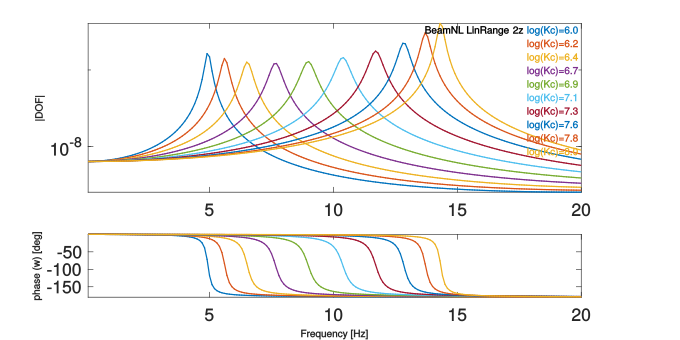
1.5.3 Definition of an underlying linear system

When defining a non-linear constitutive law, it is always possible and often desirable to define an underlying linear system. Taking the simple case of a cubic spring where s_nl=e_nl³. Figure 1.6 clearly illustrates the difference between the tangent stiffness, slope of force at current point 3 e_nl², and the secant stiffness, ratio of force divided by deformation e_nl².

Figure 1.6: Left : Tangent and secant stiffness. Right : possible underlying linear systems for the BeamNL example.

When defining a non-linear constitutive law, it useful and SDT-HBM requires that an underlying linear system be defined. For a general F_nl(e(t),ė(t)) law, the non-linear stress used in time integration should thus be of the form

(1.120)

with [k_J]{e_nl(t)} the chosen linear representation of the non-linearity and F₀ the value of the non-linear stress at the system state around which the response is computed.

When considering assembly in SDT, elements with a non-linearity defined through the NLdata field are ignored in linear assembly if NLdata.keepLin=0. For example, for a Maxwell model, reduction is best performed using the high frequency modulus. Thus a non-linear spring should be coupled with a linear spring using that high stiffness.