Non-linear constitutive laws

SDT-nlsim Contents Functions

1.3 Non-linear constitutive laws

While implementation of non-linear kinematics is fairly generic, users typically want to implement their own constitutive laws relating stresses to strains and possibly their history.

1.3.1 Laws with no internal states, principles

Constitutive laws where the stress only depends on strain and strain rate are the simplest. These laws exploit the framework provided by nl_inout for various element types.

The only thing that needs to be implemented is a .Fu function

(1.20)

During time/frequency evaluations it is essential that such evaluations be very fast, this has an impact on implementation and different strategies are implemented

tabular section 1.3.2.
dedicated user function section 1.3.6 (deprecated).
anonymous function defined with parameters section 1.3.7 (deprecated).

1.3.2 Tabular interpolation

sdtweb('_eval','d_fetime.m#BumpStop')
opt=d_fetime('timeopt dt=1e-4 tend=.1');opt.Method='Back';
model=fe_time(opt,mdl)

Multiple forms are supported. Currently a cell array of

tabulated Fu (used in nl_inout FuTable), ie 1st column is the observed strain (relative displacement), 2nd column F_u1 is the corresponding stress (load). A third column F_u2 is interpreted as a coefficient applied to computed non linear load associated to velocity (Fv) (it is used for example in bumpstops to take in account a damping with offset on the displacement). Thus s_nl=F_u1(u_nl)+F_u2(u_nl) F_v(v_nl).
When each non-linearity has 3 strains, this is interpreted as contact. You are expected to have non-linear kinematics giving strains as normal component followed by two tangent directions. Thus s₁=F_normal=F_u1(u₁) and s₂=F_Tangent1=F_u2(u₁)F_v(v₂) s₃=F_Tangent2=F_u2(u₁)F_v(v₃).
When storing constitutive laws in tabular form, it is desirable to follow the SDT curve format giving the the variable names on which the function depends in the .Xlab fields, abscissa in the .X and values in the .Y field.
numeric curve ID for a curve in the stack.
string defining a predefined law, listed using nl_spring('guilist').

For Jacobian computations by nl_spring NLJacobianUpdate, one uses xxx

Supported data input forms

BumpStop dp dp kp kp cp cp dm dm km km cm cm (a bumpstop example can be found in sdtweb t_nlspring('BumpStop'). dp is the upper gap of the bumpstop, kp the upper stiffness, and cp the upper damping, then dm km and cm the same for the lower gap. This bump stop law (as friction law) is built in nl_spring Tab which is the historical implementation : there is a known approximation, the stiffness is applied from du=dp*1.001 to du=1 (so that the slope is not exactly kp), and damping from du=dp. The same for lower gap.
Friction f f c0 c0, where f is the friction load, and c0 is a damping coefficient applied on the transition around 0 velocity (c0 is typically important). Dry frictions are known to be responsible for convergence problems.

gapCylI inner cylinder within an external sleeve.
ctcFric penalized contact and friction implementation

1.3.3 Laws with internal states

Classical rheologic model exploit internal states to account for hysteresis phenomena. E.g. The elasto-visco-plastic behavior is shown in figure 1.1

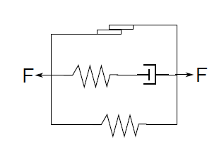
Figure 1.1: Elastic-visco-plastic model

In this case one internal state is required to represent the relative force between both extremities, to keep track of the relative displacement between the middle spring and middle dashpot.

Very complex models can be associated to this kind of representation, where one will implement internal dynamics associated to a strain history. The general formulation of such system is given as

(1.21)

and the internal states evolution equation functional

(1.22)

where {z} is a vector of internal states, {q} the displacement vector and ẋ represent the time derivatives.

Equations (1.21) and (1.22) represent the class of so-called state space models (for example in the 80's for geophysics applications, in particular by Rice and Ruina [1]).

Internal state representation can be based on the need for an efficient implementation and on the fact that the first order dynamics laws defined by equations (1.21) and (1.22) do not comply with a second order based resolution framework (the internal states acceleration is seldom defined).

Equation (1.22) can thus be resolved separately, possibly with a sub-integration scheme and an adequate interpolation of the external states.

In the non-linearity framework internal states are stored in the continuity of the generalized strains per Gauss points in field .unl. A single non-linearity only handles a single topology and a single internal model, so that each Gauss point has the same number of strain observations and internal states. The field .unl is then of size ((N_E+N_I)× N_G ) × N_T. The internal storage in field NL.unl is thus of the form

(1.23)

This formalism keeps vectorization capability per instant. The internal rate states are stored in the same manner.

Strain history is stored in the third dimension .unl(:,:,jh). In general for time integration, one will use

.unl(:,:,1) to store the current strains of the form (1.3)
.unl(:,:,2) for the initial strains u_nl0
.unl(:,:,3) to store u_nl,t−1 the strains at the previous step

When performing a residual call, it is efficient to combine time stepping (1.22) and state update. The StoreType parameters controls what the StoreState C function does.

StoreType=01 single step computation of residual and update of internal states in u_nl. The memory buffer of .unl(:,:,1) is first filled using (1.3) but assuming that internal states have not changed. The residual function computes a step replacing the data in .unl(:,:,1). StoreState (done at end of Fu) copies .snl to .FNL . Copy of internal states to unl(:,:,2) can be done by controlled by the Fu (this is in particular is done in the StoreState C++ function when upUnl2=RO.jg[2]=2 is used).
StoreType=02 stores internal states in .FNL rather than .snl.
StoreType=03 same as 01 but StoreState stores the full .snl vector followed by the full .unl(:,:,1). Beware that, this can be quite memory intensive.
StoreType=04 used for enforced motion. Modifies the displacement and velocity buffers.
StoreType=1.. if the hundreds digits is set to 1, .vnl is assumed not used and thus the associated buffer is emptied. xxx need discuss xxx

When .iopt(1)=FInd is positive, .snl is copied as a consecutive vector to model.FNL assuming the field exists. When .iopt(2)=iu is positive, internal states are copied consecutively to the displacement vector u with offset iu. This is done for Ng=.iopt(5) gauss points while skipping Nstrain=.iopt(3) components and copying Nistate=.iopt(4).

only the previous state is needed to integrate internal state evolution, as offset u_nl0 is already stored in the third dimension, u_nl,t−1 is found in the third index.

DOF representation of internal states
The number of internal states depends on the model and thus must be declared in the non-linearity. One must then declare in NLdata the fields .adofi and field .MatTyp to obtain a proper initialization of .unl field and associated observations in nl_inout.

Internal states are defined independently for each observation line used in the non-linearity. e.g. for a cbush six directions are available relative to the 3 translations and 3 rotations that can be observed. .adofi is then a line cell array of length the number of observations (6 here). Each cell defines a number of internal states associated to the corresponding observation index by providing a column vector with as many lines as internal states used each containing the DOF extension .99. The cell is left empty if no internal state is declared for a particular direction.
Thus NLdata.adofi={[];[];[];[];[];.99} will add an internal state to the 6^th observation of the non-linearity.
.99 adds the internal state as an additional DOF, while -.99 uses an FNL internal state.
Field .adofi must be either a one column vector/cell (Gauss point wise replication is supported) or should feature as many columns as expected Gauss points for the non-linearity.
For a volume element in large transformation, 9 components of stress gradient are observed. .adofi=zeros(18,1)+.99 will interlace 18 internal states with the observation at each Gauss point.

By default, one should let initialization procedures allocate DOF identifiers to each internal states by only providing a DOF extension in .adofi. If internal states have a physically defined nodal support, it is also possible to provide the corresponding DOF instead of just an extension. Beware that these DOF should not be coupled to the elastic model, as external resolution would interfere with the internal dynamics. Internal DOF replication for each Gauss point is automatically carried out if a single column is provided.

To allow clean representation and access to internal states, the global model DOF are automatically augmented with DOF associated to internal states. One can then decide whether to keep them or not during the resolution phase by setting positive (kept) or negative (eliminated) signs to the non-empty values in .adofi. To simplify for a given non-linearity all internal states are either kept or not, any negative value will then switch to elimination. In the case where internal states are kept during the resolution displacement and velocity states are automatically updated in the model.

HBM solvers specificity

HBM formulations have a resolution approach that is different from usual transient simulations that usually require to write separate dedicated functions for both resolution strategies.

In transient simulations, strain history is available, so that one first integrates internal states defined by equation (1.22), and then computes the non-linear forces with equation (1.21).

In HBM based formulations the steady state response state is assumed in the prediction/correction scheme, including strain history. Internal states coefficients are thus predicted, so that the corresponding non-linear force defined inequation (1.21) is directly obtained. One then updates the internal states evolution equation (1.22) for convergence iterations. Internal states DOF must thus be kept in the resolution phase.

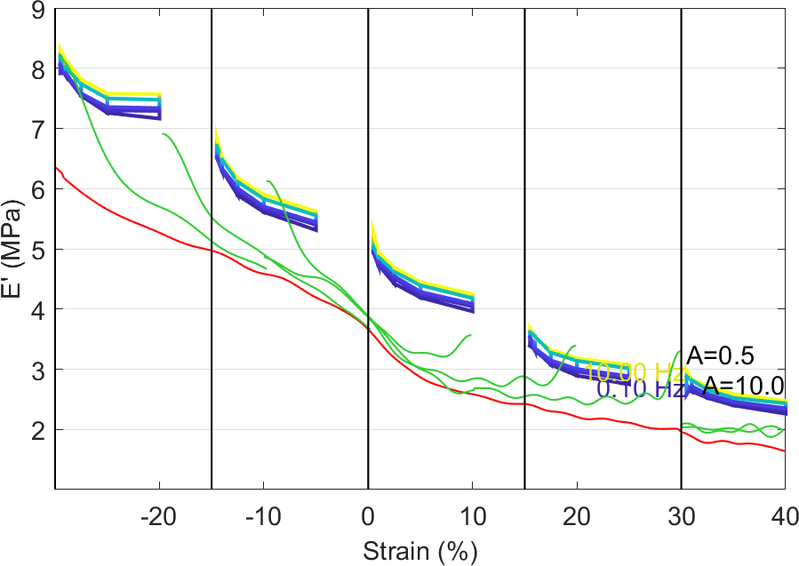
1.3.4 Hyper-visco-hysteretic 0D model

For the representation of bushings, each Gauss point is a scalar (0D) constitutive law that considers a combination of hyperelastic (red curve in figure 1.2), rate independent hysteresis (green curves from low speed triangular testing), and viscoelastic behavior (blue to yellow maps denoting frequency and amplitude dependence from sine testing).

Figure 1.2: Tangent hyperelastic stiffness (red), hysteretic relaxation modulus (green), viscoelastic complex modulus (blue to yellow)

The total load is a series of forces/stresses

(1.24)

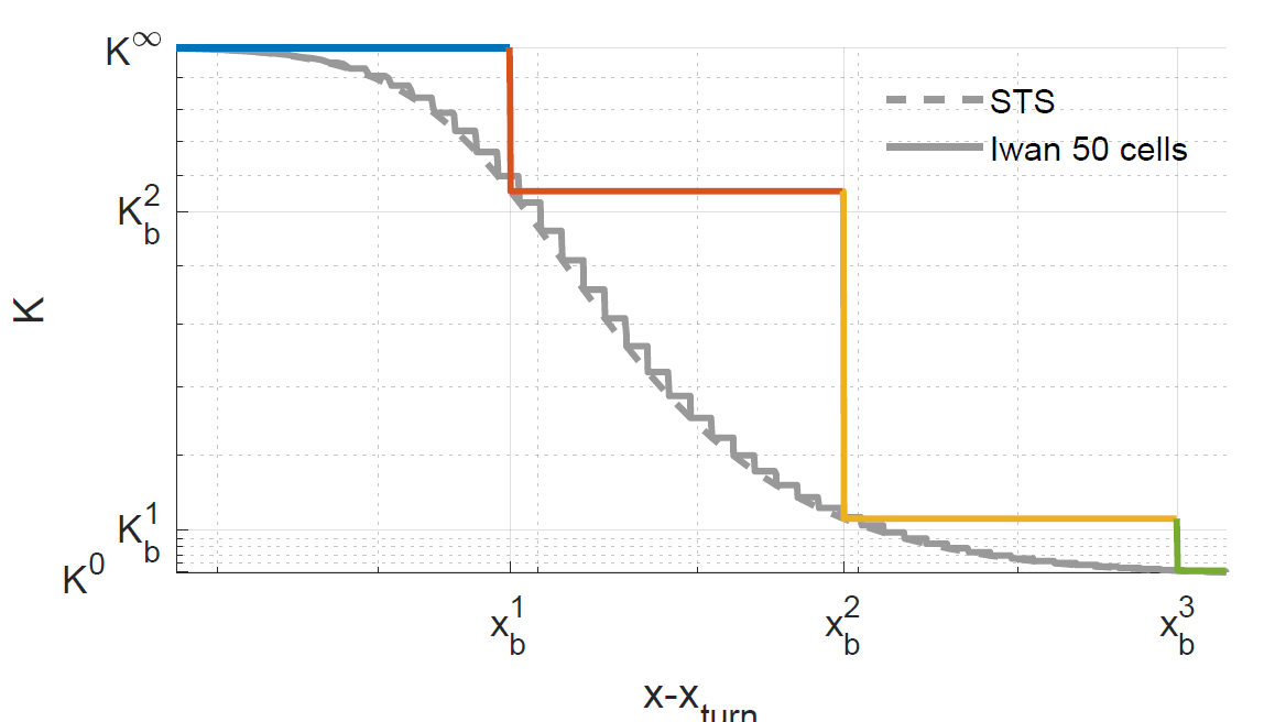
where hyperelasticity is represented using a tabular form with either linear of piecewise cubic interpolation with no internal states F_g⁰(u_g) (stored as NLdata.Fu{k})and other behavior is represented using a series of cells (also called branches in reference to the classical rheologic representation of figure 1.3), specified using a field .cell where each row describes a branch indexed by i with [ty gi fi xfi ai] type, load fraction, and if used frequency in Hz , sliding distance, non-linearity coefficient. xxx Note that the convention is to declare constants using a fraction of the high frequency modulus

g⁰+

∑

gⁱ= 1 (1.25)

but when starting relaxations from the low frequency stresses, the coefficient gⁱ/g⁰ is more relevant and that coefficient only needs to be positive.

Currently supported types

4 stress rate relaxation (adds high frequency branches) with Lion transition between viscous and hysteretic behavior (for non-zero x_fi). A relaxation frequency f_i=ωⁱ/2π=Kⁱ/(cⁱ 2π), a load fraction g_i=Kⁱ/K^∞, and a saturation distance x_fi (stored in a NLdata.Fu{k}.cell row containing [8 gi fi(Hz) 1/xfi(1/disp,strain)]) are used for the differential evolution law

(1.26)

For the linear case, the following illustrates the contributions of branches in the frequency domain.

Figure 1.3: Generalized Maxwell model and associated frequency domain response. Stress/strain rate relaxation model adds s/(s+ω_j) with non-zero high frequency contribution (orange to blue contributions in the plot).

An implicit approximation of the differential equation given by

(1.27)

leading to fixed time step increment equation

(1.28)

Alternatively an explicit approximation in Fⁱ with F⁰(t_n+1) known

(1.29)

leading to fixed time step increment equation

(1.30)

xxx recheck

1 viscoelastic relaxation of strain removes low frequency branches −gⁱ/(s/ω_j+1) from the total response. Using one internal state uⁱ associated with each Gauss point, a relaxation frequency f_i=ωⁱ/2π=Kⁱ/(cⁱ 2π) and a load fraction g_i=Kⁱ/K^∞ (stored in a NLdata.Fu{k}.cell row containing [1 gi fi(Hz) 0]), the evolution is described by

(1.31)

Note that F⁰ is here the high frequency asymptote. The implicit increment equation uses uⁱ(t_n+1)(1+ω_i dt) = ω_i dt u(t_n+1) + uⁱ(t_n) leading to

(1.32)
2 viscoelastic relaxation of strain rate (stress rate is better), internal state uⁱ

(1.33)
3 viscoelastic relaxation of hyperelastic stress, internal state Fⁱ

(1.34)
4 viscoelastic relaxation of hyperelastic stress rate, internal state Fⁱ,

(1.35)
9 Lion transition between viscous and hysteretic behavior for 3D deviatoric stress u is a scalar per material point and not by stress component.
Ḟⁱ + Fⁱ ω_i (1+β_i u) = gⁱg⁰ Ḟ⁰ (1.36)
301 For 3D hyperelastic behavior without large deformation, one assumes a reference linear elastic behavior σ=D є. The hyperelastic stress is assumed to be a function of I(є)=є₁₁+є₂₂+є₃₃ (used as an approximation of Ī₁−3 see xxx) of the form
σ₀ = f(I(є)) [D] {є}     (1.37)

the viscoelastic forces and then obtained using xxx
σⁱ + σⁱ ω_i (1+β_i u) = gⁱg⁰ σ⁰     (1.38)

and the non-linear strain contribution (where the linear contribution is removed if keepLin>0) xxx
s_nl=(g₀−1) [D]{є} +

∑

i

σⁱ     (1.39)
5 friction element (Iwan model, Jenkins cell) with simple target, parameters are sliding distance x_fⁱ=F_fⁱ/Kⁱ and load fraction g_i=Kⁱ/K^∞. The load saturation formulation with internal state corresponding to the hysteretic force Fⁱ and evolution equation

(1.40)

is preferred to the classical displacement formulation with internal state uⁱ position of last turning point,

(1.41)
6 friction element with Dahl transition using internal state Fⁱ, parameters F_fⁱ=K^∞g_i x_fⁱ limit force and speed exponent αⁱ (stored in a_i coefficient) associated with evolution equation

(1.42)
7 friction element with Dahl stress relaxation using internal state Fⁱ, parameters F_fⁱ=K^∞g_i x_Tⁱ limit force and speed exponent αⁱ (stored in NLdata.Fu{k}.g, .xf and .aDahl) xxx associated with evolution equation

(1.43)

Figure 1.4: Scheme for Iwan model and respective response in terms of hysteretic relaxation and on force/displacement domain.

For runtime integration, the data necessary for evolution equations is stored as

.opt=[ FuCode=uMax tc dt0 ] followed by a series of cell constants starting at opt(10).
.iopt starts with the standard Find, iu, Nstrain, Nistate, Ngauss(5), then a list of operations are specified starting from tcell(10) and cval=opt(10). Implemented values are listed using sdtm.enum('nlUmaxw')
- tcell=-1,cval=[] last cell
- tcell=1,cval=[v1 v2 v3] viscoelastic (Maxwell) relaxation of strain, 3 cval values give the recursion uⁱ := (uⁱv₂+ u⁰)/v₁ and load fraction definition Fⁱ=v₃ uⁱ=Kⁱ uⁱ. v₁=ω_i in rad/s, v₂=g_i/g₀, if non-zero v₃=1/x_fi.
- 2, cval=[v1 v2 v3] viscoelastic relaxation of strain, values in cval give the recursion uⁱ := (uⁱv₂+ v⁰)/v₁ and gain Fⁱ=v₃ uⁱ=Kⁱ uⁱ
- 3, cval=[v1 v2 v3] viscoelastic relaxation of stress, values in cval give the recursion Fⁱ:=(Fⁱv₂+ v₃ F⁰)/v₁.
- 4, cval=[v1 v2 v3] viscoelastic relaxation of stress rate, values in cval give the recursion Fⁱ:=(Fⁱv₂+ v₃ Ḟ⁰)/v₁. xxxLion saturation needs documenting
- Slip1D,Slip2D friction using 1 or 2 sliding directions use 4, cval=[Mu KtLin kappa dMudV Sat KtSat]]
- 101 F0_dim1 F0_dim2 interpolation table to estimate a scalar s_nl(u_nl). Supported values for dim2 are listed in sdtm.enum('nlFu') (linear, piecewise cubic, analytic forms, ...)
- 102 linear scalar stiffness, one constant
- 103 linear scalar viscosity
- tcell=[1000 unlshift snlshift] component change.
- tcell=300, cval=[c1, c2, c3, kappa, kappav] hyperelastic material cell he MooneyRivlin CiarletGeymonat
- tcell=301, cval=[omegai,gi/g0,ef] relaxation of deviatoric part of S given by Ṡⁱ+(ωⁱ+∥d∥/є_f)Sⁱ = gⁱ/g⁰ Ṡ⁰ xxx discuss (2.39) with Rafael xxx
- tcell=[400 ] xxx non usual interlacing Ng for first strain g, Ng of u_t1, u_t2,

The constants v_i depend on the integration scheme and constitutive laws

For implicit integration of Maxwell form (1.31), the evolution equation of the internal state is

(1.44)
For implicit integration of strain rate (1.33), the evolution equation of the internal state is

(1.45)
For implicit integration of stress and stress rate, simply replace u with F.

1.3.5 User callback in nl_inout, MexCb field

The current high performance developments are focusing on vectorized user implementation of non-linearities integrated in the chandle nl_inout implementation. In the data structure used during time integration (see section 1.6.3), the .MexCb field is used to provide data. It is a cell array giving {@fun,RO}.

For optimized operation limiting field name checks, the option structure RO is assumed to have ordered fields

.unlg at a single Gauss point,
.opt copy of NL.opt,
.jg int32 vector allowing passing of current Gauss point index,
.vnlg optional copy of velocities at Gauss point or empty.
.mID is initialized to the chandle/mhandle C pointer when needing a callback to modify non-linearity data.

Expected return arguments are snl and uint (new value of internal states).

1.3.6 Dedicated user function (deprecated)

The easiest conceptual way to define a non-linearity is to use your own function. For example, if you have defined the function

function NL=resCubic(NL,fc,model,u,v,a,opt,Case,RO) 
NL.unl=-.01*NL.unl.^3  ... % Cubic stiffness on relative motion
     + -.02*NL.vnl;        % Linear viscous damping on relative velocity

You can specify that this function should be used to compute a law with no internal states using

model=d_fetime('TestbeamNL');
model=nl_spring('SetPro proid100 Fu="@resCubic"',model);
% verify that Fu was defined in NLdata
NL=stack_get(model,'','NL','get');NL.NLdata.Fu
% The same with a subfunction in d_hbm
model=nl_spring('SetPro proid100 Fu="d_hbm(''@resCubic'')"',model);
NL=stack_get(model,'','NL','get');NL.NLdata.Fu

Note that in instances of deployed MATLAB generated with the MATLAB compiler, all custom functions must be defined a priori. And only anonymous functions may be created.

The NLdata entry is kept as the one defined by the nl_inout db call. Entry NLdata.Fu must then be replaced by the handle to the dedicated function in the non-linear property

1.3.7 .anonymous field for definition (deprecated)

To allow parameter edition, the base mechanism to automatically create an .Fu as MATLAB anonymous function handle is to use the following NLdata fields

.anonymous a string which upon model initialization in nl_spring('Init') will be transformed to an anonymous function of the form
Fu=@(NL,~,~,~,~,~,opt,~)AnonymousString
The @(...) part can be included in the string if it differs from the default.
Parameters are fields of the NL non-linear structure (in the example below NL.par1 will be defined). The initialization of these parameters is performed using the NLdata.Param field described below.
In frequency domain solvers, the current frequency (rad/s) is accessible in opt.w.
.csv a string to define parameters in the anonymous function. This string declares parameters using cingui ParamEdit format. This declares the parameters to be used, with a default value, their type and a possible brief explanation, as illustrated below.
.Param The current parameters. .Param can be
- a string defining the parameters declared in the .csv by par1=val1 par2=val2 ...
- a structure with fields corresponding exactly to the declared parameters struct('par1', val1, 'par2', val2).
Any omitted parameter will be set to its default declared in .csv. Lack of default values would then results in an error at the function execution.
.tex a string providing a tex format of the formula used in .anonymous.

Use of inline functions. One can directly use the existing framework with a customized call based on the concept of anonymous function handles in MATLAB.

d_hbm('TestDuffing2Dof-an')
% completes the defintion
NLdata=struct('csv','par1(1#%g#"value of parameter 1")',...
'Param','par1=val',...
'tex','p_1 u_{NL}'
'anonymous','-NL.par1*NL.unl');
model=feutil('setpro 2001',model,'NLdata',NLdata);

1.3.8 Maxwell cell model using matrices (deprecated)

The Maxwell cell model belongs to a category of so-called rheology based models. the force at each Gauss point is calculated based on an internal rheology identified as a spring-mass based model. Figure 1.5 illustrates the Maxwell (or Zener) model.

Figure 1.5: Standard viscoelastic model (single cell Maxwell or Zener). Generalized multi-cell model.

Since each branch is decoupled, one can write a series of scalar internal state evolution equations

(1.46)

and recompose the total non-linear stress using

(1.47)

To allow more general superelement representation of the constitutive law, the external force s_nlb can be defined defined by a first order equation involving the system strain state at a given Gauss point e_b and ė_b, and a series of internal states e_i and ė_i. In the following bold letters refer to non-scalar values for a given Gauss point.

(1.48)

No external forces being applied on the internal rheology, one is able to use a Schur complement to obtain the internal states evolution equation

(1.49)

Once the internal state is resolved, the external force can be deduced

(1.50)

Resolution of equation (1.49) can be obtained with different strategies. In transient simulations a local integration is performed using the Euler scheme. From instant t_n the internal state at instant t_n+1 has to be integrated over h=t_n+1−t_n

(1.51)

Implemented strategies can involve either single or multiple step integration in implicit or explicit form. Implicit resolution involves Newton-Raphson resolution, the usual initial prediction assuming constant velocity over the time step.

In the harmonic balance method, the global resolution scheme iterates on the internal states, so that one directly computes equations (1.49) and (1.50) from the current solution and the be used in the residue equation. The harmonic balance scheme then checks non-linear forces equilibrium and the stability of internal velocities.