PDF Index
| SDT-base
Contents
Functions
PDF Index |
A superelement is a model that is included in another global model as an element. In general superelements are reduced: the response at all DOFs is described by a linear combination of shapes characterized by generalized DOFs. The use of multiple superelements to generate system predictions is called Component Mode Synthesis (CMS). For a single superelement (SE structure not included in a larger model) simply use fe_reduc calls. This section addresses superelements integrated in a model.
Starting with SDT 6, superelements are stored as SE entries in the model stack (of the form 'SE', SEname, SEmodel) with fields detailed in section 6.3.2. Superelements are then referenced by element rows in a group of SE elements in the global model. A group of superelements in the Elt matrix begins by the header row [Inf abs('SE') 0]. Each superelement is then defined by a row of the form
[NameCode N1 Nend BasId Elt1 EltEnd MatId ProId EltId].
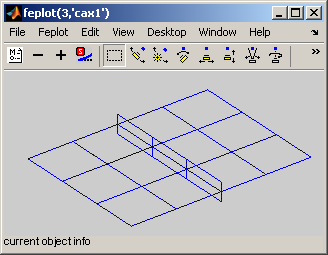
The d_cms demo illustrates the Component Mode Synthesis based on a superelement element strategy. The model of this example (shown below) is composed by two stiffened plates. CMS here consists in splitting the model into two superelement plates that will be reduced, before computation of the global model modes.
 Run
step 1 builds the simple model shown above
Run
in step 2 the two parts are separated and defined as super-elements
Run
now display
Run
step 1 builds the simple model shown above
Run
in step 2 the two parts are separated and defined as super-elements
Run
now display Other examples of superelement use are given in section 6.3.3.
The superelement data is stored as a 'SE',Name,Data entry of the global model stack. The following entries describe standard fields of the superelement Data structure (which is a standard SDT model data structure with possible additional fields).
Options characterizing the type of superelement as follows:
| Opt(1,1) | 1 classical superelements, 3 FE update unique superelements (see upcom). |
| Opt(1,4) | 1 for FE update superelement uses non symmetric matrices. |
| Opt(2,:) | matrix types for the superelement matrices. Each non zero value on the second row of Opt specifies a matrix stored in the field K{i} (where i is the column number). The value of Opt(2,i) indicates the matrix type of K{i}. For standard types see MatType. |
| Opt(3,:) | is used to define the coefficient associated with each of the matrices declared in row 2. An alternative mechanism is to define an element property in the il matrix. If these coefficients are not defined they are assumed to be equal to 1. See p_super for high level handling. |
Nominal node matrix. Contains the nodes used by the unique superelement or the nominal generic superelement (see section 7.1). The only restriction in comparison to a standard model Node matrix is that it must be sorted by NodeId so that the last node has the largest NodeId.
In the element row declaring the superelement (see above) one defines a node range N1 NEND. The constraint on node numbers is that the defined range corresponds to the largest node number in the superelement (NEND-N1+1=max(SE.Node(:,1))). Not all nodes need to be defined however.
Nodes numbers in the full model are given by
NodeId=SE.Node(:,1)-max(SE.Node(:,1))+NEND
N1 is really only used for coherence checking).
Superelement matrices. The presence and type of these matrices is declared in the Opt field (see above) and should be associated with a label giving the meaning of each matrix.
All matrices must be consistent with the .DOF field which is given in internal node numbering. When multiple instances of a superelement are used, node identifiers are shifted.
Initial model retrieval for unique superelements. Elt field contains the initial model description matrix which allows the construction of a detailed visualization as well as post-processing operations. .Node contains the nodes used by this model. The .pl and .il fields store material and element properties for the initial model.
Once the matrices built, SE.Elt may be replaced by a display mesh if appropriate.
TR field contains the definition of a possible projection on a reduction basis. This information is stored in a structure array with fields
Following example splits the 2 stiffened plane models into 2 sub models, and defines a new model with those 2 sub models taken as superelements.
First the 2 sub models are built
model=d_cms('TutoSimpleSE -s1 model;')
SE1.Node=model.Node; SE2.Node=model.Node;
[ind,SE1.Elt]=feutil('FindElt WithNode{x>0|z>0}',model); % sel 1st plate
SE1.Node=feutil('OptimModel',SE1); SE1=feutil('renumber',SE1);
[ind,SE2.Elt]=feutil('FindElt WithNode{x<0|z<0}',model); % sel 2nd plate
SE2.Node=feutil('OptimModel',SE2); SE2=feutil('renumber',SE2);
Then mSE model is built including those 2 models as superelements
mSE.Node=[];
mSE.Elt=[Inf abs('SE') 0 0 0 0 0 0; % header row for superelements
  fesuper('s_se1') 1 16 0 1 1 100 100 1 ;    % SE1
  fesuper('s_se2') 101 116 0 2 2 101 101 2]; % SE2
mSE=stack_set(mSE,'SE','se1',SE1); mSE=stack_set(mSE,'SE','se2',SE2);
feplot(mSE); fecom('promodelinit')
This is a low level strategy. fesuper provides a set of commands to easily manipulate superelements. In particular the whole example above can be performed by a single call to fesuper('SelAsSE') command as shown in the CMS example in section 6.3.3.
In this example one takes a full model split it into two superelements through element selections
model=d_cms('TutoSimpleSE -s1 model;') % get the full model
feutil('infoelt',model)
mSE=fesuper('SESelAsSE-dispatch',model, ...
  {'WithNode{x>0|z>0}';'WithNode{x<0|z<0}'});
feutil('infoelt',mSE)
[eltid,mSE.Elt]=feutil('eltidfix;',mSE);
Then the two superelements are stored in the stack of mSE. Both of them are reduced using fe_reduc (with command option -SE for superelement, and -UseDof in order to obtain physical DOFs) Craig-Bampton reduction. This operation creates the .DOF (reduced DOFs), .K (superelement reduced matrices) and .TR (reduction basis) fields in the superelement models.
Those operations can be performed with following commands (see fesuper)
mSE=fesuper(mSE,'setStack','se1','info','EigOpt',[5 20 1e3]);
mSE=fesuper(mSE,'settr','se1','CraigBampton -UseDof');
mSE=fesuper(mSE,'setStack','se2','info','EigOpt',[5 20 1e3]);
mSE=fesuper(mSE,'settr','se2','CraigBampton -UseDof');
This is the same as following lower level commands
SE1=stack_get(mSE,'SE','se1','getdata');
SE1=stack_set(SE1,'info','EigOpt',[5 50.1 1e3]);
SE1=fe_reduc('CraigBampton -SE -UseDof',SE1);
mSE=stack_set(mSE,'SE','se1',SE1);

SE2=stack_get(mSE,'SE','se2','getdata');
SE2=stack_set(SE2,'info','EigOpt',[5 50.1 1e3]);
SE2=fe_reduc('CraigBampton -SE -UseDof',SE2);
mSE=stack_set(mSE,'SE','se2',SE2);
Then the modes can be computed, using the reduced superelements
def=fe_eig(mSE,[5 20 1e3]);     % reduced model
dfull=fe_eig(model,[5 20 1e3]); % full model
The results of full and reduced models are very close. The frequency error for the first 20 modes is lower than 0.02 %.
fesuper provides a set of commands to manipulate superelements. fesuper('SEAdd') lets you add a superelement in a model. One can add a model as a unique superelement or repeat it with translations or rotations.
For CMS for example, one has to split a model into sub structure superelement models. It can be performed by the fesuper SESelAsSE command. This command can split a model into superelements defined by selections, or can build the model from sub models taken as superelements. The fesuper SEDispatch command dispatches the global model constraints (FixDof, mpc, rbe3, DofSet and rigid elements) into the related superelements and defines DofSet (imposed displacements) on the interface DOFs between sub structures.
The following strategy is now obsolete and should not be used even though it is still tested.
Superelements are stored in global variables whose name is of the form SEName. fe_super ensures that superelements are correctly interpreted as regular elements during model assembly, visualization, etc. The superelement Name must differ from all function names in your MATLAB path. By default these variables are not declared as global in the base workspace. Thus to access them from there you need to use global SEName.
Reference to the superelements is done using element group headers of the form [Inf abs('name')].
The fesuper user interface provides standard access to the different fields (see fe_super for a list of those fields). The following sections describe currently implemented commands and associated arguments (see the commode help for hints on how to build commands and understand the variants discussed in this help).
Warnings. In the commands superelement names must be followed by a space (in most other cases user interface commands are not sensitive to spaces).
make complete adds zero DOFs to nodes which have less than 3 translations (DOFs .01 to .03) or rotations (DOFs .04 to .06). Having complete superelements is important to be able to rotate them (used for generic superelements with a Ref property).
Set calls of the form fesuper('Set Name FieldOrCommand', 'Value') are obsolete and replaced as follows
All sensors, excepted resultant sensor, are supported for superelement models. One can therefore add a sensor with the same way as for a standard model with fe_case ('SensDof') commands: fe_case(model, 'SensDof [append, combine] SenType', Name, Sensor). Name contains the entry name in the stack of the set of sensors where Sensor will be added. Sensor is a structure of data, a vector, or a matrix, which describes the sensor (or sensors) to be added to model. Command option append specifies that the SensId of latter added sensors is increased if it is the same as a former sensor SensId. With combine command option, latter sensors take the place of former same SensId sensors. See section 4.7 for more details.
Following example defines some sensors in the last mSE model
% First two steps define model and split as two SE
mSE=d_cms('TutoSimpleSE -s2 mSE;')

mSE=fesuper(mSE,'setStack','se1','info','EigOpt',[5 50 1e3]);
mSE=fesuper(mSE,'settr','se1','CraigBampton -UseDof');
mSE=fesuper(mSE,'setStack','se2','info','EigOpt',[5 50 1e3]);
mSE=fesuper(mSE,'settr','se2','CraigBampton -UseDof');

Sensors={[1,0.0,0.75,0.0,0.0,1.0,0.0]; % Id,x,y,z,nx,ny,nz
 [2,10,0.0,0.0,1.0];                   % Id,NodeId,nx,ny,nz
 [29.01]};                             % DOF
for j1=1:length(Sensors);
  mSE=fe_case(mSE,'SensDof append trans','output',Sensors{j1});
end
mSE=fe_case(mSE,'SensDof append stress','output',[111,22,0.0,1.0,0.0]);
fe_case('SensMatch') command is the same as for standard models
mSE=fe_case(mSE,'SensMatch Radius2','output');
Use fe_case('SensSE') to build the observation matrix on the reduced basis
Sens=fe_case(mSE,'SensSE','output');
For resultant sensors, standard procedure does not work at this time. If the resultant sensor only relates to a specific superelement in the global model, it is however possible to define it. The strategy consists in defining the resultant sensor in the superelement model. Then one can build the observation matrix associated to this sensor, come back to the implicit nodes in the global model, and define a general sensor in the global model with the observation matrix. This strategy is described in following example.
One begins by defining resultant sensor in the related superelement
SE=stack_get(mSE,'SE','se2','GetData'); % get superelement
Sensor=struct('ID',0, ...
  'EltSel','WithNode{x<-0.5}');    % left part of the plate
Sensor.SurfSel='x==-0.5';          % middle line of the plate
Sensor.dir=[1.0 0.0 0.0];          % x direction
Sensor.type='resultant';           % type = resultant
SE=fe_case(SE,'SensDof append resultant',...
  'output',Sensor); % add resultant sensor to SE
Then one can build the associated observation matrix
SE=fe_case(SE,'SensMatch radius .6','output'); % SensMatch
Sens=fe_case(SE,'Sens','output');         % Build observation
Then one can convert the SE observation matrix to a mSE observation matrix, by renumbering DOF (this step is not necessary here since the use of fesuper SESelAsSE command assures that implicit numbering is the same as explicit numbering)
cEGI=feutil('findelt eltname SE:se2',mSE);
% implicit nodes of SE in mSE
i1=SE.Node(:,1)-max(SE.Node(:,1))+mSE.Elt(cEGI,3);
% renumber DOF to fit with the global model node numbers:
NNode=sparse(SE.Node(:,1),1,i1);
Sens.DOF=full(NNode(fix(Sens.DOF)))+rem(Sens.DOF,1);
Finally, one can add the resultant sensor as a general sensor
mSE=fe_case(mSE,'SensDof append general','output',Sens);
One can define a load from a sensor observation as following, and compute FRFs:
mSE=fe_case(mSE,'DofLoad SensDofSE','in','output:2') % from 2nd output sensor

def=fe_eig(mSE,[5 20 1e3]);     % reduced model
nor2xf(def,mSE,'acc iiplot'); ci=iiplot;