4.6  Sensor and wireframe geometry definition formats

Experimental setups can be defined with a cell arrays containing all the information relative to the sensors and wireframe geometry. This array is meant to be filled any table editor (Excel, CSV, ...), often outside MATLAB. Note you can also use the URN format in many cases section 4.6.4.

Using EXCEL you can read raw data with data=sdtacx('excel read filename',sheetnumber) or use wire=ufread('filename.xlsx') which expects the Nodes, Elements, Sensors tabs.

4.6.1  Sensors tab

The Sensors tab is mandatory and stored in MATLAB as a cell array. The first row gives column labels (the order in which they are given is free). Each of the following rows define a sensor. Known column headers are

• 'tlab' (or possibly 'lab') contains the names of the sensors. Providing a name for each sensor is mandatory. The typical format is T1:X indicating node name T1 and an indication of sensor nature X.
• 'SensId' contains the identification numbers of the sensors (will be stored in column 1 of the tdof field). Each sensor must have a unique SensId. If the identification is non integer, the integer part is taken to be a NodeId. For example 10.01 will be taken to be node 10.
• 'TestLab' can be used to specify the label used in Siemens TestLab export to .mat format (thus allowing automated reordering). This is used to build the Map:TestLab map relating acquisition channel name TestLab with desired name tlab.
• 'FEMId' can be used to specify localization and help node matching. This can also be given in a Nodes tab and will be stored in column 2 of the tdof field.
• 'X', 'Y' and 'Z' can contain the Cartesian coordinates of each sensor in the reference frame. For cylindrical coordinates replace the column headers by 'R', 'Theta' and 'Z' (mixing both types of coordinates inside the cell array is not currently supported). Such columns are mandatory except if localization is given by FEMId or if the tab Nodes described below is provided.
• 'DirX','DirY','DirZ' can be used to indicate a measurement direction.
• 'unit' can be used to specify unit label and possibly conversion. For example '*1e-3=kN' will multiply the observation by 1e-3 to obtain kN.
• 'SensType' can contain optional information such as the name of the sensor manufacturer, their types, etc.
• 'DirSpec' contains a specification of the direction in which the measurement is done at each sensor. A minus in front of any specification can be used to generate the opposite direction (-TX for example). Available entries are

  'dir x y z'	Direction of measurement specified trough its components in global coordinates (the vector is normalized).
  'X'	[1 0 0], translation in the reference frame
  'Y'	[0 1 0], in the reference frame
  'Z'	[0 0 1], in the reference frame
  'R'	unit radius translation in the cylindrical reference frame
  'THETA'	unit azimuth translation in the cylindrical reference frame
  'N'	normal to the element(s) to which the sensor is matched (automatically detected in the subsequent call to SensMatch)
  'TX'	tangent to matched surface in the N,X plane.
  'TY'	tangent to matched surface in the N,Y plane
  'TZ'	tangent to matched surface in the N,Z plane
  'TR'	tangent to matched surface in the N,R plane
  'TTHETA'	tangent to matched surface in the N,THETA plane
  'N^TX'	tangent orthogonal to the N,X plane
  'N^TY'	tangent orthogonal to the N,Y plane
  'N^TZ'	tangent orthogonal to the N,Z plane
  'N^TR'	tangent orthogonal to the N,R plane
  'N^TTHETA'	tangent orthogonal to the N,THETA plane
  'laser xs ys zs'	where (xs,ys,zs) are the coordinates of the primary or secondary source (when mirrors are used).
  'FEM 10.01'	associated FEM DOF
  'ColAct,1'	Collocated to FEM Load Act column 1.

  Additional accepted specifications for non linear time simulations (may require SDT-nlsim license). Note that the using can then also be given DirSpec using lab.{unit=*coef=ulab}.

  'PX','PY','PZ'	absolute position in the reference frame
  'rX','rY','rZ'	rotation with respect to reference frame
  'vx','vy','vz'	velocity with respect to reference frame (time derivative of 'x','y','z')
  'ax','ay','az'	acceleration with respect to reference frame (second derivative of 'x','y','z')
  'ux','uy','uz'	for springs relative motion in reference frame
  'sx1','sy1','sz1'	springs resultant on first node in frame associated with that node
  'Fx','Fy','Fz'	surface resultants require additional specification of type (either Resultant for fixed matrix elastic resultants, ZRes for non-linear resultants), the selected elements EltSel, resultant surface SurfSel. 'Corner:Fx{"Zres","eltsel","surfsel",dir,"dirvalue"}'
  'Mx','My','Mz'	Same as surface resultant but for moments.

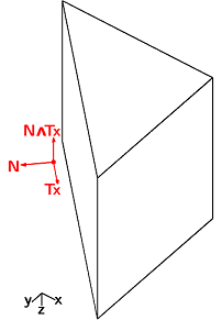
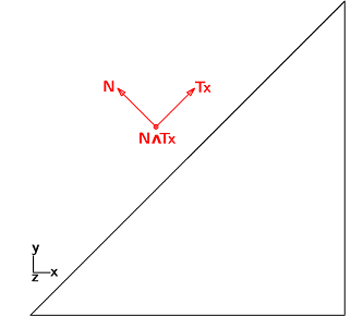
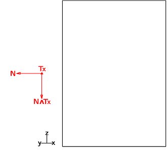
triax sensors are dealt with by defining three sensors with the same 'lab' but different 'SensId' and 'DirSpec'. In this case, a straightforward way to define the measurement directions is to make the first axis be the normal to the matching surface. The second axis is then forced to be parallel to the surface and oriented along a preferred reference axis, allowed by the possibility to define 'T*'. The third axis is therefore automatically built so that the three axes form a direct orthonormal basis with a specification such as N^T*. Note that there is no need to always consider the orthonormal basis as a whole and a single trans sensor with either 'T*' or N^T* as its direction of measure can be specified.

4.6.2  Nodes and Elements

Two optional tabs can also be provided to ease the definition of Nodes (especially when triaxes are involved) and Elements. Wireframe is then built on the fly.

Known column headers of the tab Nodes are

• 'NodeName' : node label which will be stored in nmap Map:Nodes of the wireframe for coordinates given as X, Y, Z and in nmap Map:Nodes of the model for coordinates given with FEMId.
• 'NodeId' : Identification number of the node in the wireframe geometry.
• 'FEMId' : Identification number of the FEM node used to place the sensor. This forces the use of the Sens.InFEM=1 mode, see sens.tdof. X Y Z are then ignored (only shown as information). When sensors correspond to a test setup, FEM is useful to build the wireframe (get node position with FEMId and sensor orientation with DirSpec). But it is sometimes more convenient to get back a standalone definition of sensors once positions and orientations are resolve : this is obtained with the option -InFEM2Standalone in the command fe_case('SensMatch').
• 'X' 'Y' 'Z' : X Y and Z coordinates manually given. This forces the use of the Sens.InFEM=0 mode.

Known column headers of the tab Elements are

• 'Type' : Name of the element type whose list can be found in chapter 9
• 'Nodes' : All columns on the right side from column 'Nodes' are used to give element node numbers. One row defines one element. Use as many columns as needed (for example 3 columns for tria3).

4.6.3  Example

In the example below, one considers a pentahedron element and aims to observe the displacement just above the slanted face. The first vector is the normal to that face whose coordinates are [−√2/2,√2/2,0]. The second one is chosen (i.) parallel to the observed face, (ii.) in the (x,y) plane and (iii.) along x axis, so that its coordinates are [√2/2,√2/2,0]. Finally, the coordinates of the last vector can only be [0,0,−1] to comply with the orthonormality conditions. The resulting sensor placement is depicted in figure 4.10

cf=feplot;cf.model=femesh('testpenta6');fecom('triax');
RO.Node={'NodeName','NodeId','XYZ';
'Tri'     ,1       ,[.4  .6  .5]
'Mono1'   ,2       ,[.4  .6  .1]
'Mono2'   ,3       ,'@FEM5'
'Mono3'   ,4       ,[1   0   0.5]
'Mono4'   ,5       ,'@FEM6'      };
RO.Elements={'Type' ,'Nodes';
'mass1',1      ;
''     ,2      ;
''     ,3      ;
''     ,4      ;
''     ,5      };
RO.tdof={'tlab'   ,'SensId','DirSpec'   ;
'Tri:N'  ,1.01    ,'N'         ;
'Tri:TX' ,1.02    ,'TX'        ;
'Tri:NTX',1.03    ,'N^TX'      ;
'Mono1'  ,2.01    ,'dir 1 -1 1';
'Mono2:X',3.01    ,'FEM 5.01'  ;
'Mono3:Y',4.01    ,'Y'         ;
'Mono4:N',5.01    ,'N'         };
%RO.BadSensId=[]; % to exclude bad sensors from operations
RO.EnvSensId=100;
%sens=fe_sens('tdoftable',tcell);
cf.mdl=fe_case(cf.mdl,'SensDof','Test',RO);
cf.mdl=fe_case(cf.mdl,'SensMatch radius1','Test','selface');
sdth.urn('Tab(Cases,Test){Proview,on,deflen,.2,arProp"linewidth,2"}',cf)
sens=fe_case(cf.mdl,'sens');
fe_sens('tdoftable',cf,'Test') % see summary of match results
tname=fullfile(sdtdef('tempdir'),'SensSpec.xls');
% Test write to excel to illustrate ability to reread
if ispc % Only works with ActiveX and MS-Excel at the moment
ufwrite(tname,cf.CStack{'Test'})
end

---

Figure 4.10: Typical axis definition of a triax sensor attached to a penta6

---

It is also possible to define sensor orientations and positions using only one cell array, by providing both the DirSpec and the X Y Z or FEMid position like in the example below.

model=demosdt('demo ubeam-pro');
cf=feplot; model=cf.mdl;
n8=feutil('getnode NodeId 8',model); % triax pos.
tdof={'lab','SensType','SensId','X','Y','Z','DirSpec';...
      'sensor1 - trans','',1,0.0,0.5,2.5,'Z';
      'sensor2 - triax','',2,n8(:,5),n8(:,6),n8(:,7),'X';
      'sensor2 - triax','',3,n8(:,5),n8(:,6),n8(:,7),'Y';
      'sensor2 - triax','',4,n8(:,5),n8(:,6),n8(:,7),'Z'};
sens=fe_sens('tdoftable',tdof);
cf.mdl=fe_case(cf.mdl,'SensDof','output',sens);
cf.mdl=fe_case(cf.mdl,'SensMatch radius1');
fecom(cf,'curtab Cases','output'); % open sensor GUI

4.6.4  URN based handling of sensors

URN (uniform resource names) are being used more consistently throughout SDT and the effort also applies to sensors. nl_inout slab sensors are used for time domain observation (requires SDT-nlsim license) so consistent definitions will be gradually incorporated into SDT-base.

Sensors labels should be in the format BodyName:NodeName:DirSpec when nodes are associated with different bodies or lab:DirSpec. When using repeated superelements, BodyName should be of the form SeName(index).

model = femesh('testubeamt');
%model=fe_case(model,'DofSet','Base','RB{z==0}');%DofSet not FixDof to allow resultant
model=fe_case(model,'FixDof','BaseF','z==0');
model=feutil('setmat 1 eta .02',model); % Define loss 
model=sdth.urn('nmap.Node.set',model,{'5:Base';'104:Corner'});
r1=struct('DOF',104.03,'def',1.1); % 1.1 N at node 365 direction z 
model=fe_case(model,'DofLoad','PointLoad',r1); 
model= stack_set(model,'info','Freq',70:80);
try; % Possibly download solver with ofact('patchmkl');
 model=stack_set(model,'info','oProp',mklserv_utils('oprop','CpxSym'));% change solver
end
model=fe_case(model,'sensDofInFEM','Out',{'Corner:z';'Base:Fz{Resultant,"","x==0"}'});
C1=fe_simul('DFRF -sens',model);
[sys,TR]=fe2ss('free 5 10 0',model);C2=qbode(sys,C1.X{1}*2*pi,'-struct');
iicom('curveinit',{'curve','Dfrf',C1;'curve','SS',C2})
%def=fe_simul('DFRF -sens -UseDofLoad',model);
% Reexpand partial DOF on full DOF 
dgiven=fe_def('subdof',TR,feutil('findnode z<.3',model));
mo1=fe_case(model,'DofSet','Enforced',dgiven,'remove','PointLoad');
d2=fe_simul('dfrf -matdes 1 3',stack_rm(mo1,'','Freq'));

4.6.5  Mesh cut selections

Volume cuts are often relevant to display internal motion. These commands package calls to the underlying lsutil level set handling utilities.

 model=demosdt('DemoUbeamSens NoPlot');cf=feplot(model,fe_eig(model,[5 20 1e3]))
 % Init phase   ToFace(type,Lc,AngCosMin,epsl)
 % Cut phases using y= and x= planes
cf.sel(1)='urn.SelLevelLines{Init{ToFace 1 .3 .9}}{y,.45 -.45,ByProId}{x,-.45 .0 .45,ByProId}';
feval(sdtm.feutil.MergeSel,'addTestNode',cf); % If you want to keep SensDof nodes and arrows
cf.os_('FiCutPro')
%fecom('SaveSel','@ProjectWd/selCutA.mat'); % Save selection for later reuse
% Alternate format to initialize geodesic information in SelLevelLines 
% RI=struct('Elt','selface','ToFace',[1 .3 .9]);lsutil('EdgeSelLevelLines',cf,RI)
%% Prepare for restricted superelement import, illustrated in d_cms('TutoAnsCb') 
moView=feval(sdtm.feutil.MergeSel,'Wire',cf.sel);
% Read superelement 
%RO=struct('dtype','MoKTR', ... % Form with mesh, matrices K, restitution TR
%    'RestrictTo',moView, ...  % Restrict TR to view mesh 
%    'Remove','{pl,il}');   % Remove material information 
% SE=sdtm.nodeLoadSE(FileName,RO); 
% sdtm.save('FF_SEExport.mat','SE')

Cuts use nodes placed on edges, SDT thus uses two edge nodes of the original FEM per cut node. When generating a superelement export file, the convention is to

• keep unchanged any named node or any node used in the .NeedDof field.
• if not already used reuse the node identifier of the edge node closest to the cut point.
• reuse an identifier of the superelement otherwise. TR.isCut is used to indicate that renumbering occurred.

4.6.6  Sensor GUI, a simple example

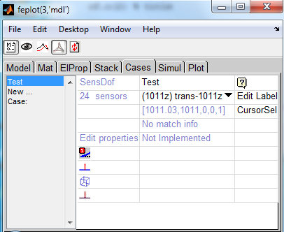
Using the feplot properties GUI, one can edit and visualize sensors. The following example loads ubeam model, defines some sensors and opens the sensor GUI.

model=demosdt('demo ubeam-pro');
cf=feplot; model=cf.mdl;
model=fe_case(model,'SensDof append trans','output',...
[1,0.0,0.5,2.5,0.0,0.0,1.0]); %  add a translation sensor
model=fe_case(model,'SensDof append triax','output',8); % add triax sensor
model=fe_case(model,'SensDof append strain','output',...
[4,0.0,0.5,2.5,0.0,0.0,1.0]); %  add strain sensor
model=fe_case(model,'sensmatch radius1','output'); % match sensor set 'output'
sdth.urn('Tab(Cases,output){Proview,on}',cf)% open sensor GUI

Clicking on Edit Label one can edit the full list of sensor labels.
The whole sensor set can be visualized as arrows in the feplot figure clicking on the eye button on the top of the figure. Once visualization is activated one can activate the cursor on sensors by clicking on CursorSel. Then one can edit sensor properties by clicking on corresponding arrow in the feplot figure.

The icons in the GUI can be used to control the display of wire-frame, arrows and links.

---

Figure 4.11: GUI for sensor edition

---