PDF Index
| SDT-rotor
Contents
Functions
PDF Index |
Once rotor model is created, one can perform time computation. nl_spring function is very useful in that case. Gyroscopic effects can be treated as non linear load depending on instant value of a model DOF (observation of the rotation speed for example). Links between fixed and rotating parts can also be modelized as non linear loads.
Following example simply computes the response to an impact on the disk, assuming that rotation speed is 1000 RPM:
 model=d_rotor('TestShaftDiskMdl'); % build simple 1D rotor

 % Define Time option and other parameters:
 opt=fe_time('TimeOpt Newmark .25 .5 0 1e-4 1e4'); % TimeOpt
 Range=struct('Omega',1000/60*2*pi);
 model=stack_set(model,'info','Range',Range);
 opt.matdes=[2 1 70];
 model=stack_set(model,'info','TimeOpt',opt);
 model=fe_rotor('TimeOptAssemble',model);

 % initial impact:
 model=fe_case(model,'DofLoad','In',...
     struct('def',1,'DOF',2.02,...
            'curve',sprintf('TestStep%.15g',opt.Opt(4)*5)));

 % Compute response:
 def=fe_time(model); iiplot(def);
Gyroscopic coupling is represented by a load −Ω(t).D(Ω=1)*V where Ω is the rotation speed and D the gyroscopic coupling matrix. That can be applied at each step of time using the DofKuva nl_spring non linearity (see sdtweb('nl_spring')).
An unbalanced mass is a load proportional to rotation speed. In the local rotating frame it can be described using nl_spring DofV non linearity.
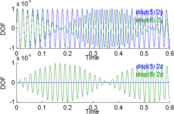
Following example deals with the simple 1D rotor and performs a time integration in fixed global frame taking in account the gyroscopic effect, for an initial impact on the disk. Note that the non linear holding of the gyroscopic effect is not necessary here since the global frame is considered, and rotation speed is assumed to be constant (1000 RPM). The gyroscopic effects (in green in figure below) are coupling the y and z motion.
 model=d_rotor('TestShaftDiskMdl');
 model=fe_case(model,'FixDof','Ends',...
           [1.01 1.02 1.03 4.01 4.02 4.03 0.01]);
 % TimeOpt:
 opt=d_fetime('TimeOpt -gamma .501');
 opt.NeedUVA=[1 1 1];
 opt.IterEnd='if ite>90;evalin(''caller'',''assignin(''''base'''',''''def'''',out)'');end';
 opt.Follow=1; opt.RelTol=-1e-5;
 opt.Opt(7)=-1; % factor type sparse
 opt.Opt(4)=1e-4; opt.Opt(5)=0.6e4; % NSteps
 % Initial impact:
 model=fe_case(model,'DofLoad','In',...
     struct('def',1e3,'DOF',2.02,...
            'curve',sprintf('TestStep%.15g',opt.Opt(4)*5)));
 % Without gyroscopic effect:
 def0=fe_time(opt,model) % compute

 % With NL gyroscopic effects:
 model=stack_set(model,'pro','DofKuva1005', ... % gyroscopic effects
     struct('il',[1005 fe_mat('p_spring','SI',1) 0 0 0 0 0],...
     'type','p_spring','NLdata',struct(...
         'type','DofKuva','lab','gyroscopic effect', ...
         'Dof',[],'Dofuva',[0 1 0],'MatTyp',70,...
         'factor',-1*1000/60*2*pi,'exponent',1,'uva',[0 1 0])));

 def=fe_time(opt,model) % compute

 % Display results as curves
 ci=iiplot;
 iicom('sub 2 1');
 iicom(ci,'IIxOnly',{'disp(1)';'disp(2)'});
 i1=fe_c(ci.Stack{'disp(1)'}.DOF,2+[.02;.03],'ind');
 iicom(ci,sprintf(';cax1;chc%i;cax2;chc%i',i1(1),i1(2)));
 % comgui('ImWrite',comgui('cd','o:\sdt.cur\rotor\plots\shaftdisk_withandwithoutgyro.png'))
 % display deformation
 cf=feplot(model); % display model
 cf.def=def0; % without gyrocopic effects
 cf.def=def;  % with gyroscopic effects
In the fixed basis the simplest bearing model is a linear spring (celas element. In rotating basis, using a spring to model beaing is not possible using a celas element. The nl_spring RotCenter non linearty is usefull to modelize link between rotating and non rotating parts.
In the fixed basis one can use a non linear spring to model the bearing. The nl_maxwell non linearity describes a set of generalized maxwell rheological models that can be used as non linear bearing in the global frame. As an illustration, following example replaces the linear bearing of the 1D rotor by a zener model of the link.
 model=d_rotor('TestShaftDiskMdl'); % Build model
 model=fe_case(model,'FixDof','Ends',...
                     [1.01 1.02 1.03 4.01 4.02 4.03 0.01]); % Clamp ends
 % TimeOpt:
 opt=d_fetime('TimeOpt');
 opt.Follow=1; opt.RelTol=-1e-5;
 opt.Opt(7)=-1; % factor type sparse
 opt.Opt(4)=1e-4; opt.Opt(5)=0.6e4; % NSteps
 opt.IterInit='model.FNL0=model.FNL+0;';
 % Initial impact:
 model=fe_case(model,'DofLoad','In',...
     struct('def',1e3,'DOF',2.02,...
            'curve',sprintf('TestStep%.15g',opt.Opt(4)*5)));
 % NL bearings
 % define nl_maxwell data
 model.il(ismember(model.il(:,1),[100;101]),:)=[]; % remove properties
 k0=500000; k1=k0/2; c1=600; % 20.41% for f=54.15 Hz
 data=nl_maxwell(sprintf('db Fu"zener k0 %.15g  k1 %.15g c1 %.15g"',k0,k1,c1));
 data.Sens{2}=3.02; % translation sensor defining nl_maxwell inputs
 r1=p_spring('default'); r1=feutil('rmfield',r1,'name');
 r1.NLdata=data; r1.il(3)=k0; % translation sensor defining nl_maxwell inputs
 r1.il(1)=100; model=stack_set(model,'pro','bearingy',r1);
 r1.NLdata.Sens={'trans',3.03}; % translation sensor defining nl_maxwell inputs
 r1.il(1)=101; model=stack_set(model,'pro','bearingz',r1);

 ci=iiplot(3); % results will be store there
 def0=fe_time(opt,model); % compute