Other information needed to specify a problem

SDT-base Contents Functions

4.5 Other information needed to specify a problem

Once the mesh defined, to prepare analysis one still needs to define

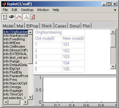
material and element properties associated to the various elements.
boundary conditions, constraints (see section 4.5.4) and applied loads (see section 4.5.5)

Graphical editing of case properties is supported by the case tab of the model properties GUI (see section 4.5.3). The associated information is stored in a case data structure which is an entry of the .Stack field of the model data structure.

4.5.1 Material and element properties

You can edit material properties using the Mat tab of the Model Properties figure which lists current materials and lets you choose new ones from the database of each material type. m_elastic is the only material function defined for the base SDT. It supports elastic materials, linear acoustic fluids, piezo-electric volumes, etc.

Figure 4.5: Material tab.

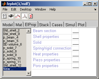
Similarly the ElProp tab lets you edit element properties. p_beam p_shell p_solid and p_spring are supported element property functions.

Figure 4.6: Property tab.

When the view mode is selected ( icon pressed), you can see the elements affected by each material or element property by selecting it in the associated tab.

You can edit properties using the Pro tab of the Model Properties figure which lists current properties and lets you choose new ones from the database of each property type (Figure 4.6).

The properties are stored with one property per row in model.il (see section 7.3) and model.il (see section 7.4). When using scripts, it is often more convenient to use low level definitions of the material properties. For example (see demo_fe), one can define aluminum and three sets of beam properties with

 femesh('reset');
 model=femesh('test 2bay plot');
 model.pl = m_elastic('dbval 1 steel')
 model.il = [ ...
 ... % ProId SecType             J      I1     I2     A
       1 fe_mat('p_beam','SI',1) 5e-9   5e-9   5e-9   2e-5  0 0 ; ...
       p_beam('dbval 2','circle 4e-3') ; ... % circular section 4 mm
       p_beam('dbval 3','rectangle 4e-3 3e-3')...% rectangular section
  ];

Unit system conversion is supported in property definitions, through two command options.

-unit command option asks for a specific unit system output. It thus expects possible input data in SI, prior to converting (and generating a proper typ value).
-punit command option tells the function that a specific unit system is used. It thus expects possible input data in the specified unit system, and generates a proper typ value.

The 3 following calls are thus equivalent to define a beam of circular section of 4mm in the MM unit system:

il = p_beam('dbval -unit MM 2 circle 4e-3'); % given data in SI, output in MM
il = p_beam('dbval -punit MM 2 circle 4'); % given data in MM, output in MM
il = p_beam('dbval -punit CM -unit MM circle 0.4'); % given data in CM, output in MM

To assign a MatID or a ProID to a group of elements, you can use

the graphical procedure (in the context menu of the material and property tabs, use the Select elements and affect ID procedures and follow the instructions);
the simple femesh set commands. For example femesh('set group1 mat101 pro103') will set values 101 and 103 for element group 1.
more elaborate selections based on FindElt commands. Knowing which column of the Elt matrix you want to modify, you can use something of the form (see gartfe)
FEelt(femesh('find EltSelectors'), IDColumn)=ID;
You can also get values with mpid=feutil('mpid',elt), modify mpid, then set values with elt=feutil('mpid',elt,mpid).

4.5.2 Other information stored in the stack

The stack can be used to store many other things (options for simulations, results, ...). More details are given in section 7.7. You can get a list of current default entry builders with fe_def('new').

 info,    EigOpt, sdtdef('DefaultEigOpt-safe',[5 20 1e3])
 info,      Freq, sdtdef('DefaultFreq-safe',[1:2])
  sel,       Sel, struct('data','groupall','ID',1)
 ...

Figure 4.7: Stack tab.

4.5.3 Cases GUI

Figure 4.8: Cases properties tab.

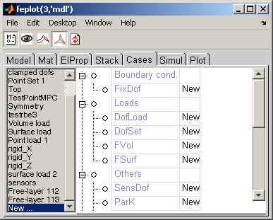
When selecting New ... in the case property list, as shown in the figure, you get a list of currently supported case properties. You can add a new property by clicking on the associated new cell in the table. Once a property is opened you can typically edit it graphically. The following sections show you how to edit these properties trough command line or .m files.

Figure 4.9: Cases properties tab.

4.5.4 Boundary conditions and constraints

Boundary conditions and constraints are described in in Case.Stack using FixDof, Rigid, ... case entries (see fe_case and section 7.7). (KeepDof still exists but often leads to misunderstanding)

FixDof entries are used to easily impose zero displacement on some DOFs. To treat the two bay truss example of section 4.1.1, one will for example use

 femesh('reset');
 model=femesh('test 2bay plot');
 model=fe_case(model, ...         % defines a new case
  'FixDof','2-D motion',[.03 .04 .05]', ...
  'FixDof','Clamp edge',[1 2]');
 fecom('ProInit') % open model GUI

When assembling the model with the specified Case (see section 4.5.3), these constraints will be used automatically.

Note that, you may obtain a similar result by building the DOF definition vector for your model using a script. FindNode commands allow node selection and fe_c provides additional DOF selection capabilities. Details on low level handling of fixed boundary conditions and constraints are given in section 7.14.

4.5.5 Loads

Loads are described in Case.Stack using DOFLoad, FVol and FSurf case entries (see fe_case and section 7.7).

To treat a 3D beam example with volume forces (x direction), one will for example use

 femesh('reset');
 model = femesh('test ubeam plot');
 data  = struct('sel','GroupAll','dir',[1 0 0]);
 model = fe_case(model,'FVol','Volume load',data);
 Load  = fe_load(model);
 feplot(model,Load);fecom(';undef;triax;ProInit');

To treat a 3D beam example with surface forces, one will for example use

 femesh('reset');
 model = femesh('testubeam plot');
 data=struct('sel','x==-.5', ...
    'eltsel','withnode {z>1.25}','def',1,'DOF',.19);
 model=fe_case(model,'Fsurf','Surface load',data);
 Load = fe_load(model); feplot(model,Load);

To treat a 3D beam example and create two loads, a relative force between DOFs 207x and 241x and two point loads at DOFs 207z and 365z, one will for example use

 femesh('reset');
 model = femesh('test ubeam plot');
 data  = struct('DOF',[207.01;241.01;207.03],'def',[1 0;-1 0;0 1]);
 model = fe_case(model,'DOFLoad','Point load 1',data);
 data  = struct('DOF',365.03,'def',1);
 model = fe_case(model,'DOFLoad','Point load 2',data);
 Load  = fe_load(model);
 feplot(model,Load);
 fecom('textnode365 207 241'); fecom('ProInit');

The result of fe_load contains 3 columns corresponding to the relative force and the two point loads. You might then combine these forces, by summing them

 Load.def=sum(Load.def,2);
 cf.def= Load;
 fecom('textnode365 207 241');