
Model verification can be a tedious task. Delving into the nitty-gritty details of finite element models of ever-growing size and complexity is seldom valued. This is especially true when the simulation already runs. It is, however, the first step to avoid the so-called Garbage In/Garbage Out shortfalls.
This first post on model verification focuses on mesh-related verifications:
- Why can “too distorted” elements lead to negative Jacobians and numerical issues?
- How to efficiently detect and address distorted elements?
- Is mesh convergence well controlled when using first order elements or reduced integration techniques?
Geometry and Jacobians
Finite elements are efficient because each “effective” element is considered as a transformation of a base one (reference topology) for which integration has been resolved.
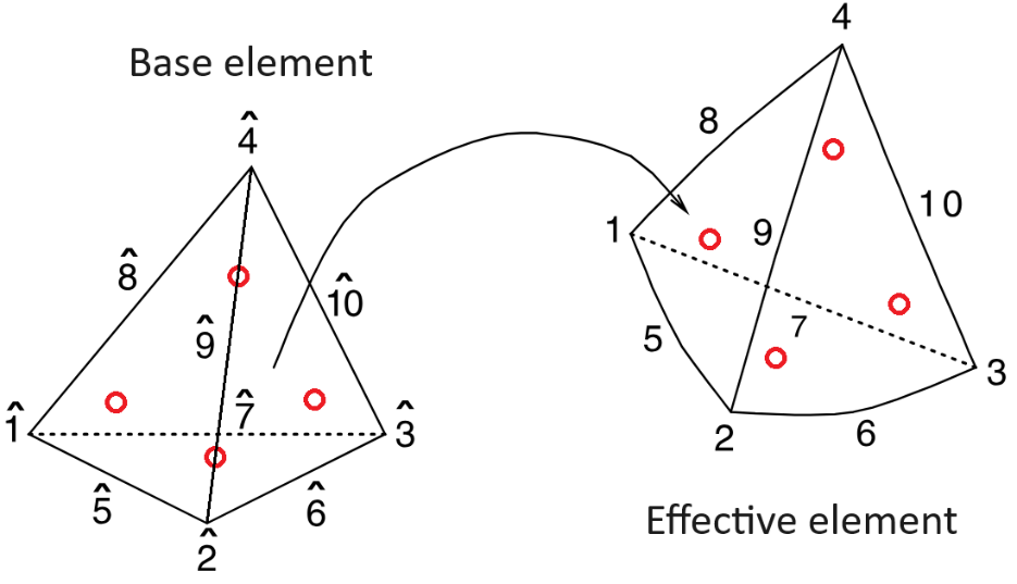
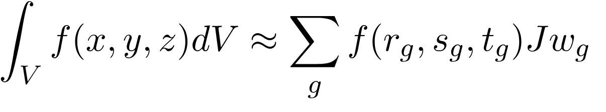
Any field (displacement, temperature, etc.) within an element volume is interpolated by shape functions (polynomials of degree equal to the element degree) and field values at element nodes. During computation, integration on the element volume is required and practically solved by summing the shape function values at Gauss points (red circles). These Gauss points are chosen with locations and weights (wg) for the summing to be equal to the full integration calculation.
This is easily achieved on each type of base elements and performed once. A coordinate transformation is then applied to each practical element to use the base element result. This leads to a Jacobian coefficient J (linked to each element volume) applied to each integration point of each element.
 You can read more in our documentation page integrules (sdtools.com).
If the element gets too far from the reference topology, the equivalence assumption does not hold and results will be impacted. In the worst case, you will get a ‘negative Jacobian’ warning or error, that will prevent the solver from running, and at least challenge its convergence.
Mesh quality checks
Computing Jacobians for all elements can be time-consuming. Controlling mesh quality is generally performed using geometry-based indicators, measuring a distortion level from the base one. Many measures exist, depending on the element and the code employed. SDT functionality fe_quality (https://www.sdtools.com/help/fe_quality.html) provides many indicators depending on the need.
Some indicators are common to all elements, such as aspect ratios, measuring the ratio between the longest edge and the shortest edge of an element. For each geometry, dedicated indicators also exist. The following illustration shows:
- Aspect ratio on a hexahedron
- Wrap on a quadrangle (measure of coplanarity, as more than 3 vertices are present).
- Interior Angle Measure for shells or volume faces
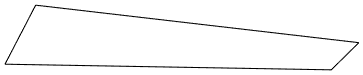
- Sliver for tetrahedron, a flatness measure of the maximum ratio between each surface against opposite summit height.
Aspect ratio 4 (against 1)
Wrap 0.017
(against 0)
max interior angle 126
(against 90)
Sliver 24.5
against 2.45)
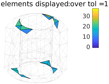
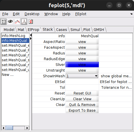
More measures are present, such as the GammaK indicator used by ABAQUS for tetrahedra. All available indicators can be displayed in an interface to assess model quality and localize potential problems.
A direct Jacobian measure is costlier but will directly highlight critical elements, with negative Jacobians responsible for execution errors. SDT will warn you about negative Jacobians and try to proceed. NASTRAN can do the same when deactivating the GEOMCHECK option. ABAQUS will try to move nodes to recover positive Jacobians with the risk of creating other convergence problems or exit otherwise.
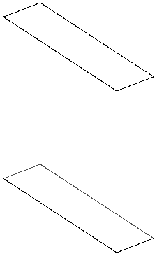
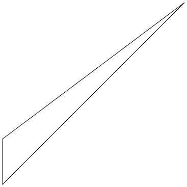
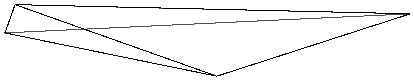
A usual workaround is to simply deactivate these elements to proceed, but some cases can be handled in a lighter way. For example, a common issue occurs with second order elements fitted on curves. The edges middle nodes do not lie on the straight line linking its extremities, resulting in a distortion. This is measured with our UnstraightEdge indicator. If the middle node is too far, you may get negative Jacobians even if the element volume itself is positive, as for the extruded pentahedron below with a minimal Jacobian of -0.2.
First order elements and reduced integration
Beyond distorted element geometry, using first-order elements can generate non-converged results for computationally affordable mesh sizes. As they are faster to resolve, some tricks exist to render a more compliant behavior, but it comes at the cost of mesh convergence control. Two techniques come to mind:
- Reduced integration. Using fewer Gauss points to compute the reference element makes the response more flexible, but it also generates hourglass modes: internal deformation without energy. Using one Gauss point at the center of gravity of an element is thus commonly used in ABAQUS with elements C3D*R, and accessible with integration rule -1 in SDT. Unless all vertices are constrained by consistent formulations, a specific hourglass control is necessary (not present in SDT). Mesh convergence becomes non-monotonous, and stiffness can be underestimated. As each code uses its own implementation, portability to other codes is seldom obtained.
- Enriched formulations. Adding shape functions to the first-order formulation (named incompatible shapes or bubble functions) improves convergence, accessible in ABAQUS with the C3D*I elements, and in SDT with integration rule 10002. As the formulation is incomplete, the improvement may be inconsistent and depends on the deformation direction. The additional cost to convergence makes it rarely interesting compared to second-order elements.
We would advise using second order elements as soon as results must be properly converged. The example below, extracted from a squeal study, illustrates the limitations of such modified first order element formulations regarding quality. We have a car suspension arm coupled to the car body through a rubber mount. The arm is finely meshed with second order tetrahedra, and the rubber layer was meshed with first order hexahedra, a surface-based constraint couples both volumes.
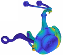
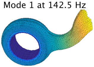
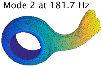
The fact that the rubber is much softer than the arm induces seemingly realistic results whatever the formulation. The connection flexibility is however greatly impacted by the chosen formulation, along with the suspension modes frequencies. In particular, the first 6 modes are the rigid arm movement on the rubber mount.
Several formulations have been tested:
– 1c. First order mesh with a refined constrained surface coupling.
– 1cI. First order mesh with bubble functions and a refined constrained surface coupling.
– 1cR. First order mesh with reduced integration and a refined constrained surface coupling.
– 1k. First order mesh with default coupling strategy.
– 1kI. First order mesh with a bubble functions and default coupling strategy.
– 1kR. First order mesh with a reduced integration and default coupling strategy.
– 2k use of a second order mesh and a refined surface coupling for the rubber taken as a reference.
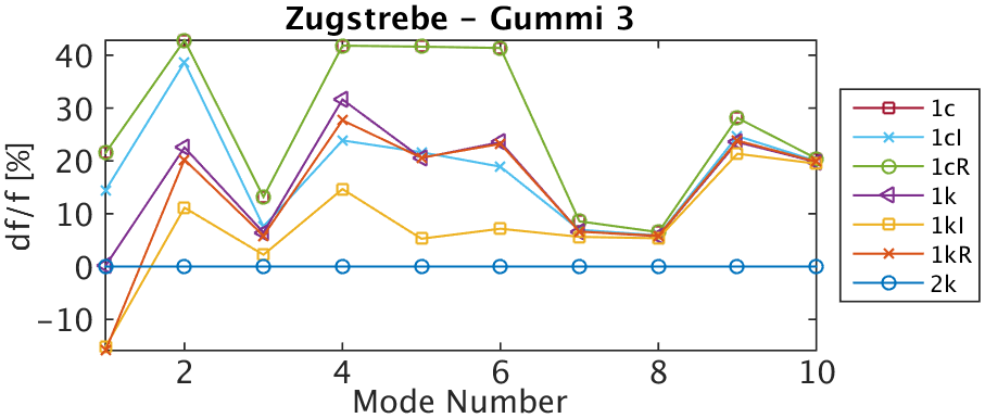
In such case, that is far from optimal but common in industrial models, variations of at least 10% are found when using first order elements. Formulation alternatives do not uniformly improve the behavior, and can become too soft.
Conclusion
Mesh elements quality regarding distortion, adapted integration and convergence is the first step of model verification. It ensures that we have a sane working base, avoiding early numerical problems. The study of mechanical assemblies goes further with the implementation of structural interactions, links and fasteners, that are often simplified using structural elements. We will discuss these aspects in the next post of our model verification series.