
How to verify that the connections in a mechanical assembly behave as intended?
The increase of computational power allows considering very large and complex assemblies. The use of connection features, as discussed in our previous post Coupling for mechanical assemblies is widespread, with many available definition and input strategies.
As part of our model verification series, following Model verification for quality assessment – Mesh level, this post focuses on mechanical assembly checks:
- Which tools to perform global assembly checks?
- How to organize detailed assembly checks through a standardized strategy ?
👉 Component/connection formalism - How to check component consistency?
👉 Components rigid body modes - How to check connection consistency?
👉 Coupled subassembly rigid body modes - How to check connection kinematics?
👉 Principal directions of relative movements between coupling components
Global checks
Once assembly features have been implemented in more or less automated ways, verification is a mandatory step. Multiple Points Constraints (MPC) have some shortcomings, and it is easy to miss specific options for DOF selection. Specifications can also be inappropriate regarding the simplified physics, input errors, or the formulation itself!
To ensure model quality, SDT implements several strategies that can be used for verification. At low level, utilities are present to check and translate MPC.
- From a generic MPC, cleanup and slaves can be resolved using command feutil FixMPCMaster
- RBE3 can be revised and checked with the commands documented in fe_case rbe3
- Consistency can be checked with fe_caseg RBCheck that will test rigid body motion
In a more general approach, computing modes, checking rigid body modes frequencies and strain energy localization around connections is a good way of ensuring consistency.
Assembly assumptions and component/connection formalism
For larger assemblies, a systematic approach is required, and full system computation times can become costly. Preliminary analyses should thus be preferred. The analysis tools developed in our SDT-CMT module allow some refined analysis illustrated on an industrial brake.
Upon defining components as element sets, the assembly can be organized as a series of components linked by connections. It is possible in this process to convert some connections to penalization. The proposed analysis detects structural kinematic chains, defined as series of connected structural elements representing a mechanism between components. The chain is then considered as a single coupling feature.
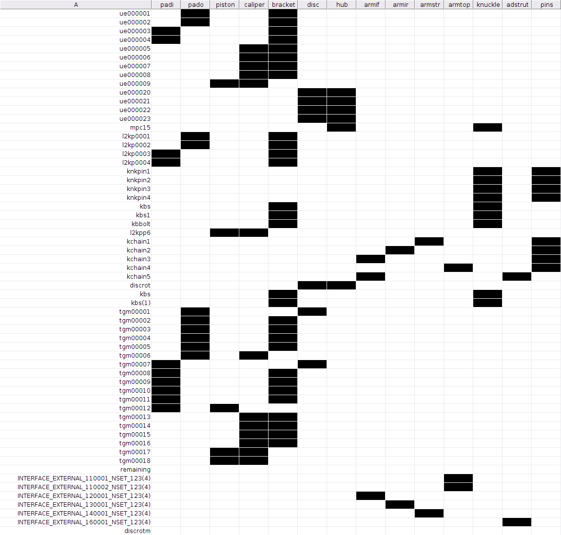
A connection table first allows mapping component connections and their associated names. The table is simple with black cells on components targeted by each connection. It can be sorted for each component. The objective is to check direct implementations and recover connections’ names to point in case of problems.
Component consistency
Coherence checks start by verifying components rigid body modes. They should be independent when extracted from the assembly. As components can internally contain constraints, this is not always a trivial task. For this purpose, one considers independent parts in each component and verify the stiffness associated to the theoretical rigid body mode subspace. The table below shows the component list, number of rigid body modes, number of independent part and the rigid body mode maximum frequency.

Here all components have 6 rigid body modes, the ‘pins’ selection target several intermediate connectors considered outside components for design purpose.
Connection consistency
A common shortcoming exists for bonded surfaces, offsets between the flanges may generate momentum transmission and compromise rotational rigid body modes, with associated frequencies possibly getting over several kHz. The model kinematics then becomes inappropriate. ABAQUS proposes for example an adjust option for this matter to ensure that no offset exists between the bonded nodes. The adjust procedure illustrated below, can be problematic for mesh exports, and can lead to undesired distortions.
In SDT an offset can exist between solids as the rotations are estimated using the translations (see feutilb.html MpcFromMatch). This ensures a good connection consistency as described in this post.
The next check concerns connection consistency. It is here verified that connections do not alter subassembly rigid body modes. Coupled components are thus extracted with their connections and theoretical rigid body modes are tested against the model. The result is the following table showing for each component connected pairs the maximum frequency obtained. The cell becomes red if a threshold of 10Hz is passed. The indication shows up to what frequency a biased rigid body motion will significantly interfere if correction cannot be directly proceeded.
Connection kinematics
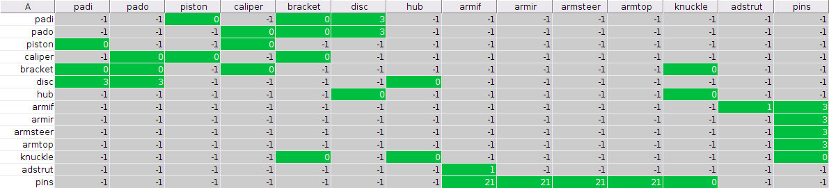
The last check concerns connection kinematics. It characterizes the principal relative movements of coupled components. Some connections are meant to represent a moving mechanism such as bearings, pivots, sliders… These connections should then generate additional rigid body modes when considering the extracted subassembly focused on the link. This is tested by checking the rigid body modes of one component of the subassembly against a rigid counterpart. One thus observes the number of free relative movements between the components and can recover the associated stiffness.
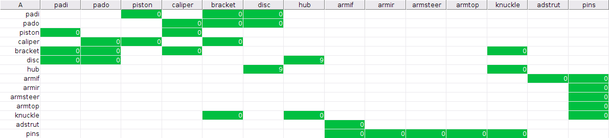
The first table shows for each component pair the number of free relative movements between components, to ensure that the obtained kinematics are coherent. For example, in the table below, ball joint connections between pins and arms show 3 free directions.
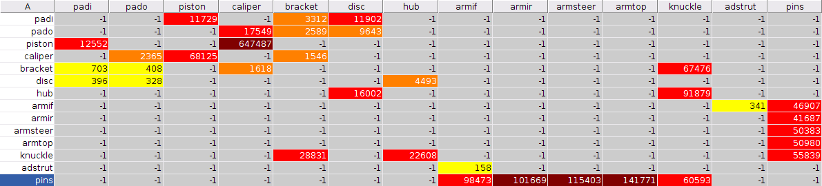
The second table displays the frequency of the first non-free relative movements. It allows assessing the connection flexibility with regards to the component mass and inertia. Over the displayed frequency one cannot consider the connection rigid anymore. This can be intended for flexible mechanisms, and then allow checking if input values are coherent. In our example, connections between the disc and pads seem soft, following a low pressure preload with a soft non-linear contact law.
For debugging matters all these coupling rigid body modes can be displayed and saved in an automated report. One can then point to specific behaviors in case of doubt by observing the principal connection directions. The following illustrations shows the bearing coupling of a hub on a knuckle free rotation movement, and a bad case of pad free slipping coupling on a disc, probably due to an error in the normal definition.
Example of principal coupling directions estimated by the connection kinematics checking procedure
Conclusion
Mechanical assembly models are now very common for FEA, but verification methods often remain ad hoc or very basic. Over traditional strategies, this post presents a systematic approach used in SDT-CMT. It directly considers resolved connections as used by the solver and characterizes their influence on several sets of rigid body modes. That way, consistency can be evaluated with no assumption on the expected behavior. Recovery of principal relative displacement allow checking the kinematics. Frequency indicators eventually provide an estimation of the connection stiffness with regards to the assembly inertia.