PDF Index
|
Contents
Functions
PDF Index |
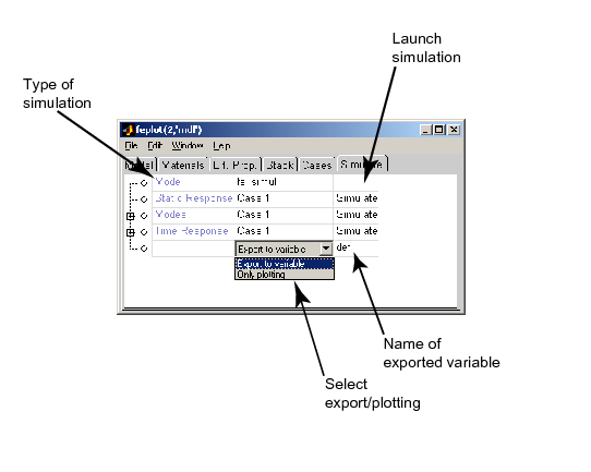
Access to standard solvers is provided through the Simulate tab of the Model properties figure. Experienced users will typically use the command line equivalent to these tabs as detailed in the following sections.
The computation of the response to static loads is a typical problem.
Once loads and boundary conditions are defined in a case as shown in previous sections, the static response may be computed using the fe_simul function.
This is an example of the 3D beam subjected to various type of loads (points, surface and volume loads) and clamped at its base:
 model=demosdt('demo ubeam vol'); % Initialize a test
 def=fe_simul('static',model');% Compute static response
 cf=feplot; cf.def=def;% post-process
 cf.sel={'Groupall','ColorDataStressMises'}
Low level calls may also be used. For this purpose it is generally simpler to create system matrices that incorporate the boundary conditions.
fe_c (for point loads) and fe_load (for distributed loads) can then be used to define unit loads (input shape matrix using SDT terminology). For example, a unit vertical input (DOF .02) on node 6 can be simply created by
  model=demosdt('demo2bay');  Case=fe_case(model,'gett'); %init
  % Compute point load
  b = fe_c(Case.DOF,[6.02],1)';
In many cases the static response can be computed using Static=kr \b. For very large models, you will prefer
kd=ofact(k); Static = kd\b; ofact('clear',kd);
For repeated solutions with the same factored stiffness, you should build the factored stiffness kd=ofact(k) and then Static = kd \b as many times are needed. Note that fe_eig can return the stiffness that was used when computing modes (when using methods without DOF renumbering).
For models with rigid body modes or DOFs with no stiffness contribution (this happens when setting certain element properties to zero), the user interface function fe_reduc gives you the appropriate result in a more robust and yet computationally efficient manner
Static = fe_reduc('flex',m,k,mdof,b);
fe_eig computes mass normalized normal modes.
The simple call def=fe_eig(model) should only be used for very small models (below 100 DOF). In other cases you will typically only want a partial solution. A typical call would have the form
 model = demosdt('demo ubeam plot');
 cf.def=fe_eig(model,[6 12 0]);  % 12 modes with method 6
 fecom('colordata stress mises')
You should read the fe_eig reference section to understand the qualities and limitations of the various algorithms for partial eigenvalue solutions.
You can also load normal modes computed using a finite element package (see section 4.3.2). If the finite element package does not provide mass normalized modes, but a diagonal matrix of generalized masses mu (also called modal masses). Mass normalized modeshapes will be obtained using
ModeNorm = ModeIn * diag( diag(mu).^(-1/2) );
If a mass matrix is given, an alternative is to use mode = fe_norm(mode,m). When both mass and stiffness are given, a Ritz analysis for the complete problem is obtained using [mode,freq] = fe_norm(mode,m,k).
Note that loading modes with in ASCII format 8 digits is usually sufficient for good accuracy whereas the same precision is very often insufficient for model matrices (particularly the stiffness).
A typical application of SDT is the creation of input/output models in the normal mode nor, state space ss or FRF xf form. (The SDT does not replicate existing functions for time response generation such as lsim of the Control Toolbox which creates time responses using a model in the state-space form).
The creation of such models combines two steps creation of a modal or enriched modal basis; building of input/output model given a set of inputs and outputs.
As detailed in section 4.8.3 a modal basis can be obtained with fe_eig or loaded from an external FEM package. Inputs and outputs are easily handled using case entries corresponding to loads (DofLoad, DofSet, FVol, FSurf) and sensors (SensDof).
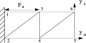
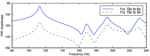
For the two bay truss examples shown above, the following script defines a load as the relative force between nodes 1 and 3, and translation sensors at nodes 5 and 6
 model=demosdt('demo2bay');
 DEF=fe_eig(model,[2 5]);  % compute 5 modes

 % Define loads and sensors
 Load=struct('DOF',[3.01;1.01],'def',[1;-1]);
 Case=fe_case('DofLoad','Relative load',Load, ...
              'SensDof','Tip sensors',[5.01;6.02]);

 % Compute FRF and display
 w=linspace(80,240,200)';
 nor2xf(DEF,.01,Case,w,'hz iiplot "Main" -reset');
You can easily obtain velocity or acceleration responses using
 xf=nor2xf(DEF,.01,Case,w,'hz vel plot');
 xf=nor2xf(DEF,.01,Case,w,'hz acc plot');
As detailed in section 6.2.3, it is desirable to introduce a static correction for each input. fe2ss builds on fe_reduc to provide optimized solutions where you compute both modes and static corrections in a single call and return a state-space (or normal mode model) and associated reduction basis. Thus
 model=demosdt('demo ubeam sens -pro');

 model=stack_set(model,'info','Freq',linspace(10,1e3,500)');
 model=stack_set(model,'info','DefaultZeta',.01);

 [SYS,T]=fe2ss('free 6 10',model); %ii_pof(eig(SYS.a),3)

 qbode(SYS,linspace(10,1e3,1500)'*2*pi,'iiplot "Initial" -reset');
 nor2xf(T,[.04],model,'hz iiplot "Damped" -po');
computes 10 modes using a full solution (Eigopt=[6 10 0]), appends the static response to the defined loads, and builds the state-space model corresponding to modal truncation with static correction (see section 6.2.3). Note that the load and sensor definitions where now added to the case in model since that case also contains boundary condition definitions which are needed in fe2ss.
The different functions using normal mode models support further model truncation. For example, to create a model retaining the first four modes, one can use
 model=demosdt('demo2bay');
 DEF=fe_eig(model,[2 12]);  % compute 12 modes
 Case=fe_case('DofLoad','Horizontal load',3.01, ...
              'SensDof','Tip sensors',[5.01;6.02]);
 SYS =nor2ss(DEF,.01,Case,1:4);
 ii_pof(eig(SYS.a)/2/pi,3)  % Frequency (Hz), damping
A static correction for the displacement contribution of truncated modes is automatically introduced in the form of a non-zero d term. When considering velocity outputs, the accuracy of this model can be improved using static correction modes instead of the d term. Static correction modes are added if a roll-off frequency fc is specified (this frequency should be a decade above the last retained mode and can be replaced by a set of frequencies)
 SYS =nor2ss(DEF,.01,Case,1:4,[2e3 .2]);
 ii_pof(eig(SYS.a)/2/pi,3,1)  % Frequency (Hz), damping
Note that nor2xf always introduces a static correction for both displacement and velocity.
For damping, you can use uniform modal damping (a single damping ration damp=.01 for example), non uniform modal damping (a damping ratio vector damp), non-proportional modal damping (square matrix ga), or hysteretic (complex DEF.data). This is illustrated in demo_fe.
NEED TO INTRODUCE PROPER REFERENCES XXX
To perform a full order model time integration, one needs to have a model, a load and a curve describing time evolution of the load.
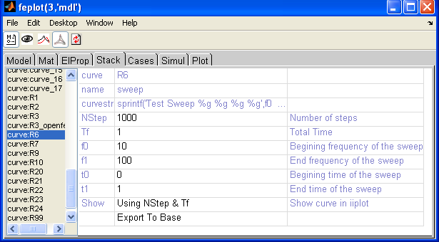
 % define model and load
 model=fe_time('demo bar');fe_case(model,'info')
 % Define curves stack (time integration curve will be chosen later):
 % - step with ones from t=0 to t=1e-3, 0 after :
 model=fe_curve(model,'set','input','TestStep t1=1e-3');
 % - ramp from t=.1 to t=2 with final value 1.1;
 model=fe_curve(model,'set','ramp','TestRamp t0=.1 tf=2 Yf=1.1');
 % - Ricker curve from t=0 to t=1e-3 with max amplitude value 1:
 model=fe_curve(model,'set','ricker','TestRicker t0=0 dt=1e-3 A=1');
 % - Sinus (with evaluated string depending on t time vector) :
 model=fe_curve(model,'set','sinus',...
               'Test eval sin(2*pi*1000*t)');
 % - Another sinus definition, explicit curve (with time vector,
 %   it will be interpolated during the time integration if needed)
 model=fe_curve(model,'set','sinus2',...
     struct('X',linspace(0,100,10)',...
     'Y',sin(linspace(0,100,10)'))); % tabulated
 % - Have load named 'Point load 1' reference 'input'
 %   curve (one can choose any of the model stack
 %   curve from it stack entry name) :
 model=fe_case(model,'SetCurve','Point load 1','input');

 cf=feplot(model) % plot the model
Once model is plotted in feplot one can edit each curve under the model properties Stack tab. Parameters can be modified. Curve can be plotted in iiplot using the Show pop-up button. One has to define the number of steps (NStep) and the total time to be displayed (Tf) and click Using NStep & Tf. One can also display curve on the info TimeOpt time options by clicking on Using TimeOpt.
One can change the curve associated to the load in the Case tab.
% Define time computation options : dt=1e-4, 100 time steps
cf.Stack{'info','TimeOpt'}=...
     fe_time('timeopt newmark .25 .5 0 1e-4 100');
% Compute and store/display in feplot :
cf.def=fe_time(cf.mdl);
figure;plot(cf.def.data,cf.def.def(cf.def.DOF==2.01,:)); % show 2.01 result
Time domain responses can also be obtained by inverse transform of frequency responses as illustrated in the following example
model=demosdt('demo ubeam sens');DEF=fe_eig(model,[5 10 1e3]);

w=linspace(0,600,6000)';                      % define frequencies
R1=nor2xf(DEF,.001,model,w,'hz struct');      % compute freq resp.
R2=ii_mmif('ifft -struct',R1);R2.name='time'; % compute time resp.
iiplot(R2);iicom(';sub 1 1 1 1 3;ylin');      % display
The flexibility given by the MATLAB language comes at a price for large finite element computations. The two main bottlenecks are model assembly and static computations.
During assembly compiled elements provided with OpenFEM allow much faster element matrix evaluations (since these steps are loop intensive they are hard to optimize in MATLAB). The sp_util.mex function alleviates element matrix assembly and large matrix manipulation problems (at the cost of doing some very dirty tricks like modifying input arguments).
Starting with SDT 6.1, model.Dbfile can be defined to let SDT know that the file can be used as a database. In particular optimized assembly calls (see section 4.8.8) make use of this functionality. The database is a .mat file that uses the HDF5 format defined for MATLAB >= 7.3.
For static computations, the ofact object allows method selection. Currently the most efficient (and default ofact method) is the multi-frontal sparse solver spfmex. This solver automatically performs equation reordering so this needs not be done elsewhere. It does not use the MATLAB memory stack which is more efficient for large problems but requires ofact('clear') calls to free memory associated with a given factor.
With other static solvers (MATLAB lu or chol, or SDT true skyline sp_util method) you need to pay attention to equation renumbering. When assembling large models, fe_mk (obsolete compared to fe_mknl) will automatically renumber DOFs to minimize matrix bandwidth (for partial backward compatibility automatic renumbering is only done above 1000 DOF).
The real limitation on size is linked to performance drops when swapping. If the factored matrix size exceeds physical memory available to MATLAB in your computer, performance tends to decrease drastically. The model size at which this limit is found is very much model/computer dependent.
Finally in fe_eig, method 6 (IRA/Sorensen) uses low level BLAS code and thus tends to have the best memory performance for eigenvalue computations.
Note finally, that you may want to run MATLAB with the -nojvm option turned on since it increases the memory addressable by MATLAB(version <=6.5).
For out-of-core operations (supported by fe_mk, upcom, nasread and other functions). SDT creates temporary files whose names are generated with nas2up('tempnameExt'). You may need to set sdtdef('tempdir','your_dir') to an appropriate location. The directory should be located on a local disk or a high speed disk array. If you have a RAID array, use a directory there.
The handling of large models, often requires careful sequencing of assembly operations. While fe_mknl, fe_load, and fe_case, can be used for user defined procedures, SDT operations typically use the an internal (closed source) assembly call to fe_case Assemble. Illustrations of most calls can be found in fe_simul.
[k,mdl,Case,Load]=fe_case(mdl,'assemble matdes 1 NoT loadback',Case); return the stiffness without constraint elimination and evaluates loads.
[SE,Case,Load,Sens]=fe_case(mdl,'assemble -matdes 2 1 3 4 -SE NoTload Sens') returns desired matrices in SE.K, the associated case, load and sensors (as requested in the arguments).
Accepted command options for the assemble call are